Project Elara 2024 research and development report
An end-of-year overview of research conducted by Project Elara
Abstract
Project Elara is a nonprofit dedicated to being part of creating a future powered by plentiful space-based solar power. In this year, the Project developed its first proposal for a prototype solar capture, microwave conversion, and transmission (SCMCT) system. System design considerations for this system are described, and initial modeling of the SCMCT system with simulation results is shown. Furthermore, a strategy for prototype testing to validate and extend upon current research is outlined.
Overview
The Sun is a star, a nuclear furnace with a power output[1] of Mamajek et al., 2015. Meanwhile, Earth’s global power consumption[2] in 2019 was IEA, 2021, 14 orders of magnitude below the power output of the sun. Even the most powerful artificial fusion reactor could hardly match the 4.6 billion-year-old, 2 trillion-quadrillion-ton one at the center of the Solar System. However, Earth-based solar power, while highly successful, has not truly delivered on the full possibilities of harnessing the energy of the Sun.
The primary difficulties of space-based solar power are twofold. First, high upfront costs and the difficulties of launching space infrastructure present immense hurdles. Second, the technological capabilities that would allow the full realization of space-based power to the point it is worth the cost are not yet possible. Therefore, the ultimate goal of the present research is to contribute towards the development of a space-based power transmission system that provides:
- Sustained high-power, high-gain wireless transmission with very low power loss
- Precision long-distance transmission capability, up to interplanetary distances
- Autonomous operation capability with robust failure resistance, multiple layers of redundancy, and assured safety
- All-weather reliability, including maintaining constant reception of power regardless of space weather and varied conditions in Earth’s atmosphere
It is without a doubt that the technologies involved in this system are far from reaching readiness. However, Abiri et al. (2022) have already demonstrated small-scale versions of this technology in low-Earth orbit. This research intends to supplement present achievements in the field with further advances in realizing space-based power.
Theoretical analysis and results
Due to the difficulties of practical testing, a theoretical model of wireless power capture and transmission was first developed for initial analysis. The conceptual system consists of mirrors and satellites situated in highly eccentric geosynchronous orbits. The individually-spaced mirrors form a composite parabolic solar collector, concentrating sunlight to a fixed point. A secondary mirror at the foci of the composite collector, segmented and also of parabolic design, directs the focused light into specialized transmitter satellites. These satellites then transmit the power to Earth in the form of microwaves. The system is planned to be only one of many, with the intent to build a space-based stellar power collection swarm around geosynchronous and eventually higher orbits which may one day be able to provide all the energy for the Earth. A simplified diagram of the system is shown in Figure 1.
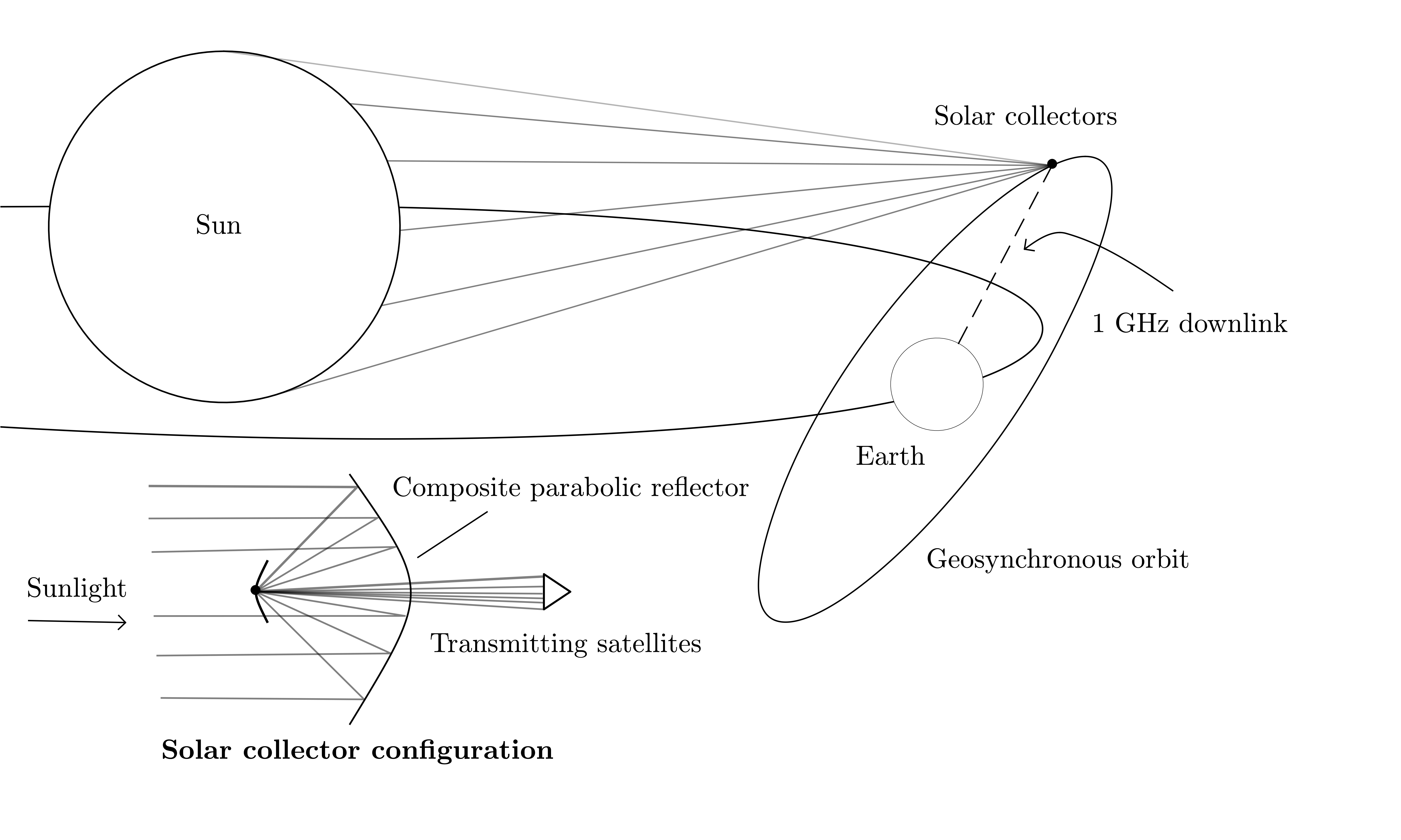
Figure 1:An illustration of a portion of the conceptual SCMCT system
For the theoretical modelling, the special case of Maxwell’s equations in free space, namely the 3D electromagnetic wave equation, was used. The electromagnetic wave equation is given by:
The proposed power transmission system operates at a frequency of 1 GHz, which has been identified as a candidate frequency for microwave power transmission due to its low atmospheric attenuation ITU-R, 2022. On initial testing, it was found that numerical simulations of the electromagnetic wave equation exhibited rapid temporal oscillations that resulted in numerical instabilities. Therefore, the time-independent variant of the electromagnetic wave equation was used instead. As is well-known, this is obtained by the separation of variables of the electromagnetic wave equation, upon the simplifying assumption that the time variation of the electric field follows . This results in the Helmholtz equation:
From this point on, only the expressions for the electric field are written and it is implied that the same expressions are true for the magnetic field up to the replacement . The Helmholtz equation was prepared in variational form (weak form) for obtaining a numerical solution by the finite element method. By multiplication with a test function , integrating over the simulation domain , and simplifying via the Divergence Theorem, one obtains the general variational form:
Where : is the double dot product (tensor contraction for matrices).
The boundary conditions must then be incorporated for a meaningful solution. As a starting case, the boundary conditions are given as follows:
Where, respectively:
- The boundary of the (primary) parabolic reflector, which reflects (and thereby focuses) the waves, with the parabolic dish centered at position ; the composite collector is modelled as an approximately solid parabolic dish with perfectly reflective (Neumann) boundaries.
- The boundary (“box”, referring to the rectangular simulation volume) of the 3D space surrounding the antenna, where waves can pass freely into and out of the region; is a small but nonzero value representing the decay of the waves as they propagate away to infinity. This boundary is not explicitly written out but is present in the transformed boundary conditions mentioned later.
- The boundary of the secondary reflector, which reflects focused light to direct it to a central collection point through an opening in the back of the parabolic dish.
- The boundary which is the opening at the bottom of the parabolic dish, where the concentrated light is directed towards the transmitting satellites. This is also not explicitly written out as it is directly encoded into the geometry of the primary reflector.
The open boundary condition is approximated by a technique described in Frei (2015), in which a coordinate transform is applied to extend the domain out to infinity, where and are respectively half the length and width of the domain bounding box. This approximately replicates an open boundary that allows outgoing electromagnetic waves to radiate outwards in all directions. Upon application of the boundary conditions, we obtain the weak form for our boundary-value problem, as given by:
The derivation of this is found in Appendix A, which is separately available. Simulations were done with the FreeFEM++ software Hecht, 2012 with a custom FreeFEM-based solver. This solver was written in the FreeFEM language and utilizes FreeFEM++'s built-in finite-element solver and mesh discretizer, but otherwise is completely custom and tailored to the specific simulation parameters. A solution in transformed coordinates was first obtained, before the built-in polynomial interpolation was used to transform the solution to coordinates, as shown in Figure 2 and Figure 3. The domain was discretized straightforwardly by assuming a simple geometry of the antenna as a perfect paraboloid, as shown in Appendix B.
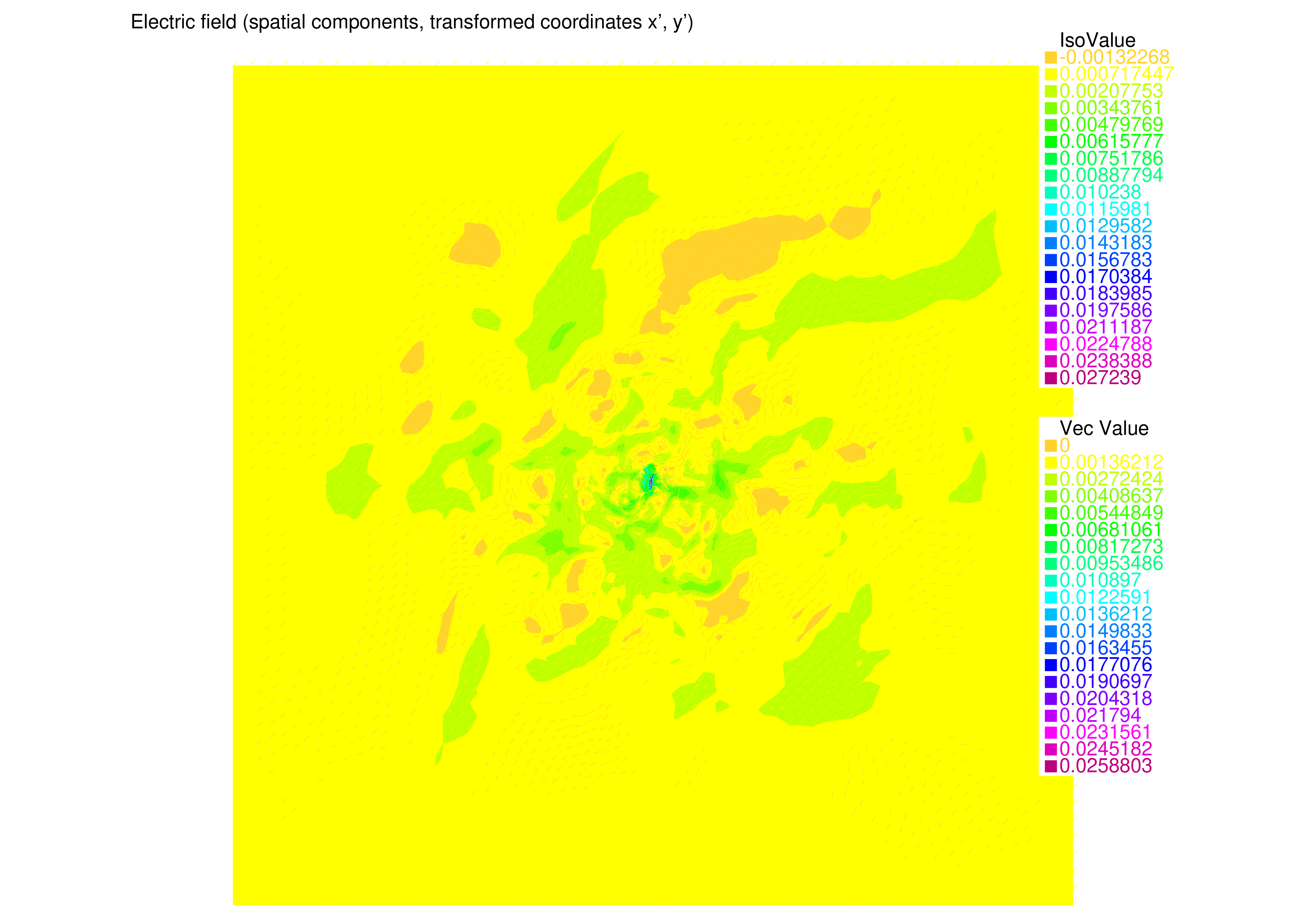
Figure 2:FreeFEM numerical solution in transformed coordinates .
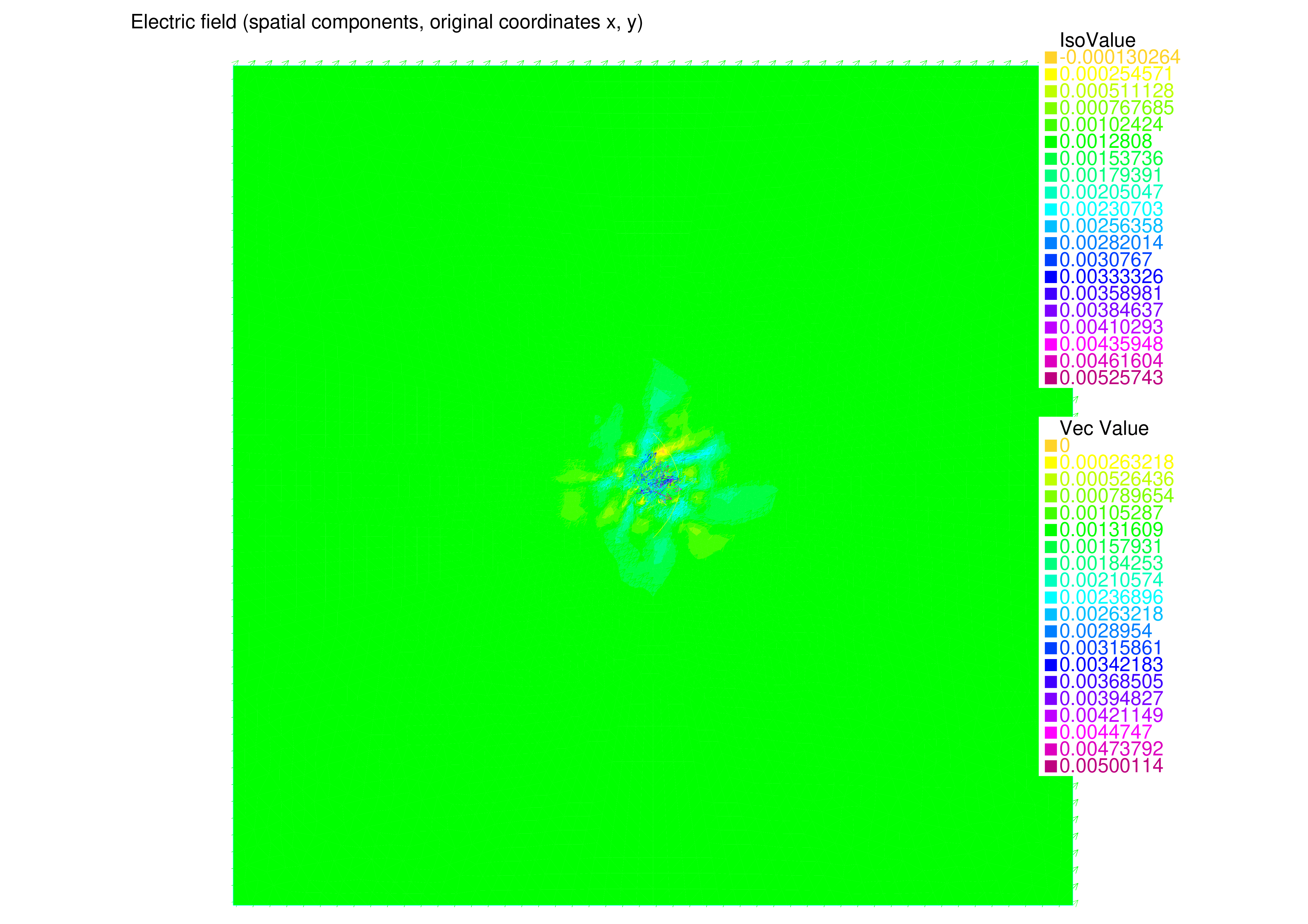
Figure 3:FreeFEM numerical solution in physical-space coordinates .
The simulation was intended as a proof-of-concept and thus it should be emphasized that the simulation results were not of specific significance and should not be intended as research data. However, several distinctive and possibly promising features did emerge out of the initial simulation. The electric field strength being highest approximately between the parabolics, and decaying quickly outside of the immediate vicinity, corresponds with the expected result. However, it should be noted that the rather weak field variation, in which the differences of the highest and lowest field strengths is merely , does not provide sufficient support for these claims. Thus these are merely deduction from observations and cannot be proven at present without further testing.
As a separate test of the fidelity of the results, a custom FreeFEM-based solver was tested against a finite-difference simulation in a similar but much simpler Helmholtz boundary-value problem. A solver written with the Python findiff library Baer, 2018, a library that implements finite difference methods for PDEs, was tested, alongside a slightly different finite-difference solver that used findiff for simply derivative discretization. The two solvers differed at most by and as such the rest of the finite-difference solution results are given by that of the primary findiff solver. The validation test took the form of solving the scalar-valued Helmholtz equation on the unit square , with the following boundary conditions, which may appear simple, but can be shown to yield a non-trivial solution:
A FreeFEM-based solver, similar although not identical to the aforementioned fully-featured vector solver, was compared against the findiff solver. The results from both simulations are shown in Figure 4 and Figure 5.
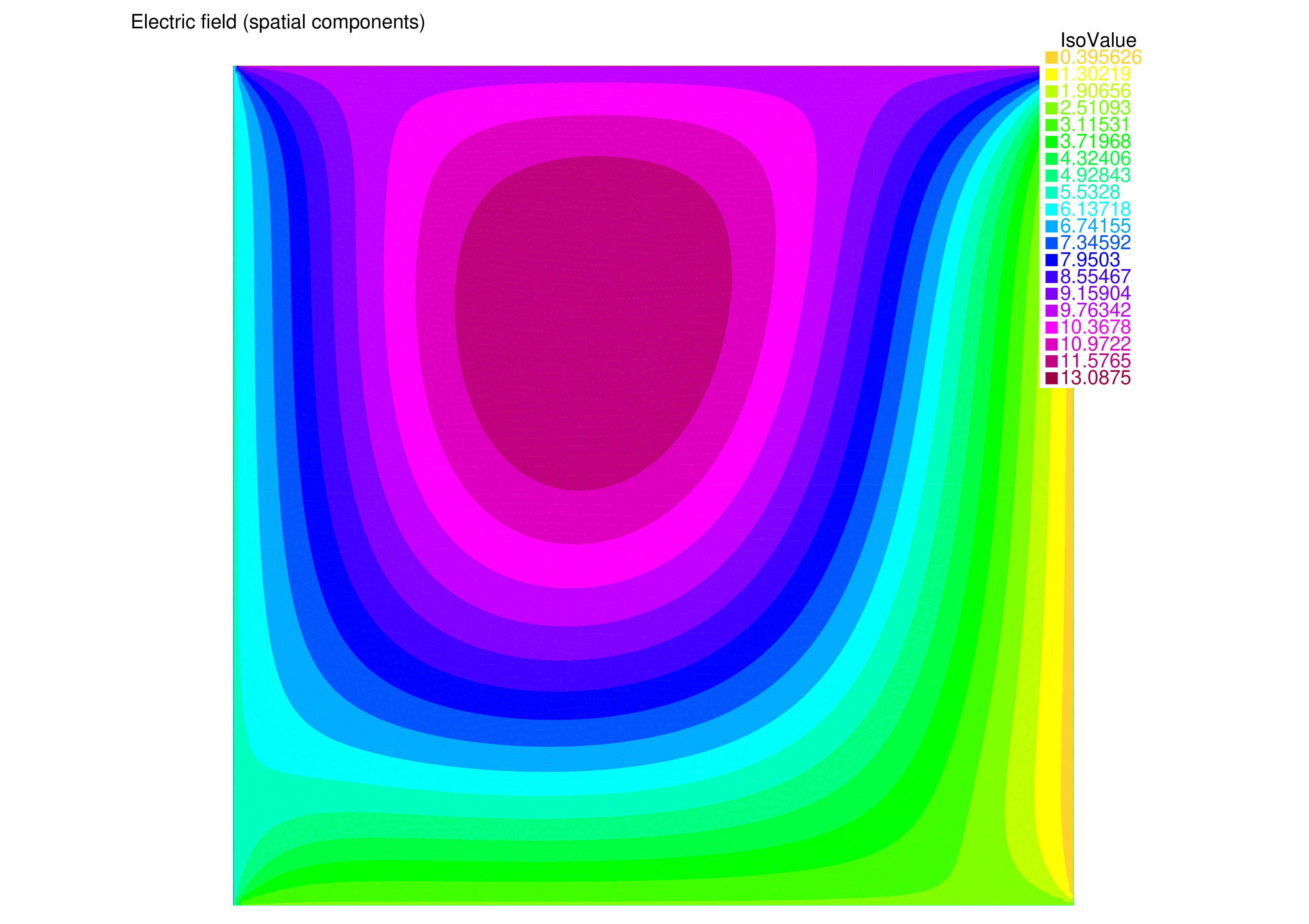
Figure 4:Numerical solution obtained by FreeFEM-based (finite element) solver.
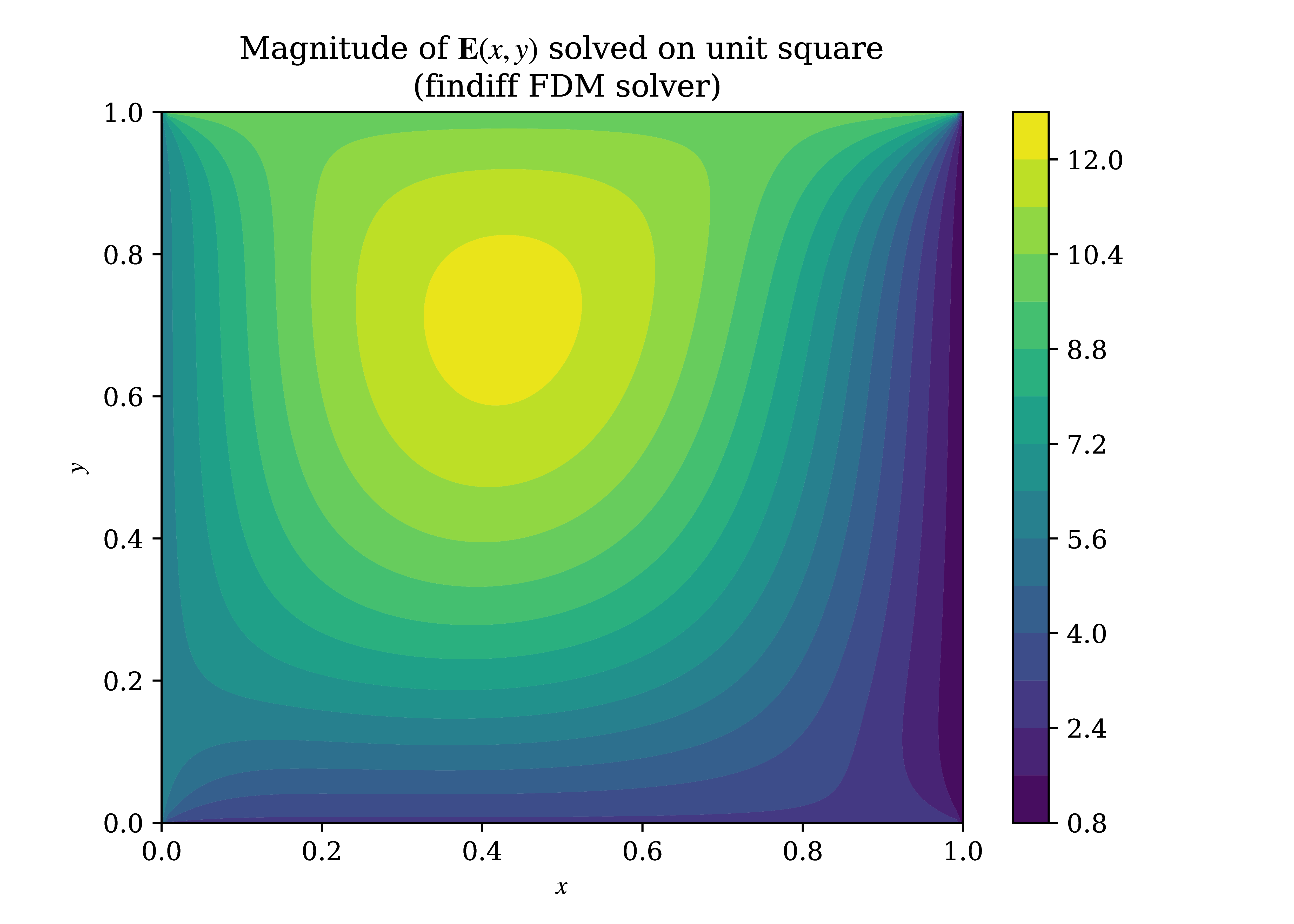
Figure 5:Numerical solution obtained by findiff (finite-difference) solver.
Comparison of the numerical solutions from the two solvers showed excellent agreement and the completion of an important intermediary diagnostic for the primary FreeFEM-based solver. Diferences between the two solutions showed almost zero difference on a number of test points evaluated from both solutions, as shown in Figure 6.
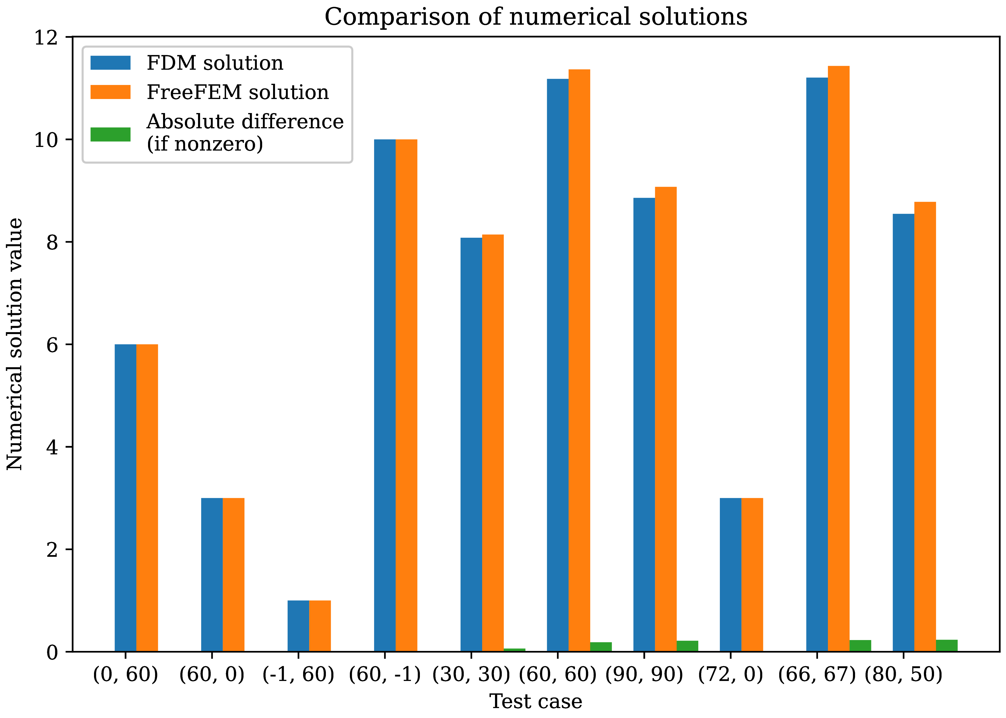
Figure 6:Comparison between numerical solutions obtained by FreeFEM and findiff-based solvers
The results suggest that the solver shows promise, at least to the extent of present testing. However, the author would like to note that a further validation test of the vector-valued Helmholtz equation has not been successfully completed as of the time of writing. Difficulties with performing an inverse coordinate transformation from the finite-difference numerical solution have yet to be resolved, among other issues. Two different methods have been attempted, that of polynomial interpolation as well as a neural network fit, but both do not meet research standards and much further work is necessary. In addition, it was found that the order of integrals was a significant factor in deciding the result of the solution, as well as the sign convention used, where there were significantly different values when changed. It is believed to be a result of the conventions of the FreeFEM++ software, but should continue to be investigated.
Planned upcoming research
Further theoretical work, including a more thorough treatment of the power collection system and theoretical modelling of the power transmission system, is necessary for advancing the research. More detailed studies of orbits and spacecraft design are also hoped for in upcoming work. In addition, construction and testing of physical prototypes to augument computational simulations is also essential. Prototypes are intended to be assembled via 3D printed components treated with electroless plating to form a smooth, metallic coating, after which specific tests may be performed. The verification of such prototypes in an experimental setting is highly anticipated to be carried out in the near future.
Disclosures
The authors would like to acknowledge the assistance of using LLMs as a source of valuable knowledge and an educational tool. No part of this paper was taken in whole or in part from content provided by the use of such tools. In addition, the author acknowledges the great assistance provided by the FreeFEM++ software documentation, including its many examples which included example solvers of the Helmholtz equation. Another excellent reference was the website of Nicolás Guarín-Zapata[3], whose work on finite-difference methods on infinite domain was invaluable in the course of this research.
Open access statement
This paper is released into the public domain and the author withdraws all rights to this work, in accordance Project Elara guidelines. For more details about the project, please see the Project Elara website.
Acknowledgments
On behalf of Project Elara and as the author of this paper, I would like to acknowledge the numerous contributions that went into this research. The support and collaborative effort of the entire Project team was essential to all of the research’s successes. Milo played a key role in providing engineering insight, Luke in mathematical and physical analysis, Charles in offering fresh suggestions and ideas, Max (Emilliano) in continual work on research, and Arnar and Nicholas for their immense enthusiasm. I would also like to thank Professor Persans and Professor Newberg of Rensselaer Polytechnic for their support, knowledge, and their generously-offered resources, and Professor Tysoe for valuable information on the suggestion of electronless plating. I thank the support of my family and friends, including Gabrielle for her valuable suggestions of emphasizing the distinctive features of the project. Finally, I thank Dr. Harold White of Limitless Space Institute and Dr. Andrew Bramante of Greenwich High School for their invaluable mentorship and guidance in the early days of my research.
According to the IAU defined value of the solar luminosity , after rounding.
Found through averaging the provided 2019 global power consumption figure of 22,848 TWh IEA, 2021 over one year.
- Mamajek, E. E., Prsa, A., Torres, G., Harmanec, P., Asplund, M., Bennett, P. D., Capitaine, N., Christensen-Dalsgaard, J., Depagne, E., Folkner, W. M., Haberreiter, M., Hekker, S., Hilton, J. L., Kostov, V., Kurtz, D. W., Laskar, J., Mason, B. D., Milone, E. F., Montgomery, M. M., … Stewart, S. G. (2015). IAU 2015 Resolution B3 on Recommended Nominal Conversion Constants for Selected Solar and Planetary Properties.
- IEA. (2021). Electricity Information: Overview [Techreport]. International Energy Agency.
- Abiri, B., Arya, M., Bohn, F., Fikes, A., Gal-Katziri, M., Gdoutos, E., Goel, A., Gonzalez, P. E., Kelzenberg, M., Lee, N., Marshall, M. A., Roy, T., Royer, F., Warmann, E. C., Vaidya, N., Vinogradova, T., Madonna, R., Atwater, H., Hajimiri, A., & Pellegrino, S. (2022). A Lightweight Space-based Solar Power Generation and Transmission Satellite.
- ITU-R. (2022). Attenuation by atmospheric gases and related effects [Recommendation ITU-R P.676-13]. International Telecommunications Union (Radiocommunication Sector).
- Frei, W. (2015). Using Perfectly Matched Layers and Scattering Boundary Conditions for Wave Electromagnetics Problems.
- Hecht, F. (2012). New development in FreeFem++. J. Numer. Math., 20(3–4), 251–265.
- Baer, M. (2018). findiff Software Package. https://github.com/maroba/findiff