Lagrangian and Hamiltonian mechanics

Newton’s laws and conservation of energy are two approaches to solving for the equations of motion of an object. We can make Newtonian mechanics more elegant by extending them to fields and potentials. But ultimately, Newtonian mechanics is still cumbersome to use. Here is an alternate, more beautiful approach - Lagrangian mechanics.

Lagrangian Mechanics

The Lagrangian is the difference of an object’s kinetic and potential energies, and is denoted by:

\[ \mathcal{L(x, \dot x)} = K(\dot x) - U(x) \]

Note that the dots are used for the time derivatives - that is, \(\dot x = \frac{dx}{dt}\). The action is a fundamental quantity of all physical systems and is given by the time integral of the Lagrangian:

\[ S = \int_{t_1}^{t_2} \mathcal{L}(x, \dot x)~dt \]

The principle of stationary action states that for any given system, the action is stationary. What does stationary mean? Recall the idea of stationary points in calculus - which include minima and maxima. For the action to be stationary, that means the Lagrangian must be a stationary function, which are analogous to stationary points, just for the action, which is a function of functions (what we call a functional, which we’ll go more in-depth with later).

But what form does that Lagrangian have to take to obey the principle of stationary action? The short answer is that it must obey the following equation, known as the Euler-Lagrange equation:

\[ \frac{\partial \mathcal{L}}{\partial x} - \frac{d}{dt} \frac{\partial \mathcal{L}}{\partial \dot x} = 0 \]

where again, \(\dot x = \dfrac{dx}{dt}\) is the velocity. This is one of the most fundamental and profound equations of physics, and works for any particle’s Lagrangian (particle, remember, can be a big object like a planet or star, it is a generic term in physics). Once you write down the Euler-Lagrange equation, you just need to take the derivatives of the Lagrangian and substitute to get the equations of motion (the differential equations you use to solve for the trajectory of the particle). Applying it, at least conceptually, is fairly simple.

But to gain a deeper understanding of why this equation works, we must first dive into the theory of functionals and variational calculus. If this section is too math-heavy, feel free to skip this section - it’s not required for applying the Euler-Lagrange equation. But for those that want the step-by-step derivation - let’s dive in!

Functionals

A functional is a function that takes in other functions as input. In contrast to a function \(f\) which takes in a real number \(x\) and outputs \(f(x)\), a functional \(\mathcal{L}\) takes in a function \(y(x)\) and outputs \(\mathcal{L}(y(x), y'(x), x)\).

The derivative appearing in \(\mathcal{L}(y, y', x)\) and the mention of the word “calculus” suggests that functionals are based in differential operators, such as derivatives and integrals. Indeed, this is the case - a great number of functionals are in fact integrals.

Consider, for instance, a functional that appears - under a different name - in a first introduction to calculus. This is the functional expression for the arc length:

\[ S = \int_a^b \sqrt{1 + {y'}^2}\, dx \]

While an introductory treatment of calculus may simply give this formula with the provided function \(y\) and its derivative \(y'\), the calculus of variations would consider this formula a functional of an arbitrary function \(f\) in the form:

\[ S(y, y', x) = \int_a^b \sqrt{1 + {y'}^2}\, dx \]

The calculus of variations is concerned with optimizing functionals to find their stationary points. In many cases, we want to obtain the minimum or maximum of a funtional, but remember that stationary points are more general and can include things like saddle points and other points of inflection (i.e. points around which the second derivative changes sign).

In our case, we want to figure out which path \(y(x)\) is the shortest distance between points \(x = a\) and \(x = b\). Translated to mathematical terms, we can say that we want to optimize \(S(y, y', x)\) for the function \(y(x)\) that minimizes \(S\). But how do we do so? The answer requires a fair bit of explaining, so this is a section to be read through slowly.

The general functional optimization problem

Consider a general functional \(S(f, f', q)\) where the functional \(S\) is a function of \(f(q)\), \(f'(q)\), and \(q\). Here, \(f(q)\) is a parametric function of one parameter \(q\) - we will explore specific cases of \(f(q)\) later (hint: one of these will be the position function \(x(t)\) which is a parametric function where the parameter is \(t\)). Our functional \(S(f, f', q)\) is given by:

\[ S(f, f', q) = \int_{q_1}^{q_2} \mathcal{L}(f, f', q)\, dq \]

All of this is certainly very abstract, so let us examine what it all means. \(S\) is a functional, meaning that it takes some function \(f(q)\) and outputs a number. The precise thing it does, in this case, is to integrate any composite function of \(f\), its derivative \(f'(q)\), and its input \(q\), between two points in the domain of \(f\). For notational clarity, we call this composite function of \(f\), \(f'\), and \(q\) as \(\mathcal{L}(f, f', q)\). As we are taking the integral of the composite function, this results in a number, since definite integrals return a number. So to sum it all up, \(S\) is a functional, that, given any function \(f(q)\) - whatever the function may be - returns the definite integral of any possible composite function of \(f\), its derivative \(f'\), and its input \(q\).

We want to find the function \(f\) that minimizes or maximizes \(S\). This means we want to find a function for which \(S\) does not change with respect to \(f\) (similar to how the derivative is zero at a critical point in normal calculus). To find this optimal function, let us vary \(S\) by adding a function \(\eta(q)\) multiplied by a tiny number \(\varepsilon\) to \(f\) between \(q_1\) and \(q_2\) - this represents adding a tiny shift, also called a variation, to \(S\). Our particular shift is such that \(\eta(q_1) = \eta(q_2) = 0\), meaning that \(\eta(q)\) vanishes at the endpoints, since we want this variation to only be between \(q_1\) and \(q_2\) (and nowhere outside of that range). We then have:

\[ S(f + \varepsilon \eta, f' + \varepsilon \eta', q) = \int_{q_1}^{q_2} \mathcal{L}(f + \varepsilon \eta, f' + \varepsilon \eta', q)\, dq \]

Our next step is to find the amount of change \(\delta S\) between \(S(f, f', q)\) and \(S(f + \varepsilon \eta, f' + \varepsilon \eta', q)\). As a first step, we want to compute \(\mathcal{L}(f + \varepsilon \eta, f' + \varepsilon \eta', q)\), as that will allow us to compute \(S(f + \varepsilon \eta, f' + \varepsilon \eta', q)\), which we need in order to calculate \(\delta S\).

We use \(\delta S\) instead of \(dS\) or \(\partial S\) as (1) \(\delta S\) is specifically for functionals and (2) the latter two symbols already have (multiple) reserved uses and we don’t want to muddle up the notation and make the meanings unclear.

Recall how, in single-variable calculus, we can express a small shift \(y(x + h)\) in a function \(y(x)\) for some tiny number \(h\) by:

\[ y(x + h) = y(x) + y'(x) h \]

This idea can be generalized to multivariable calculus, where we can express a small shift in a function \(f(x + \sigma, y + \lambda)\) in a function \(f(x, y)\) by:

\[ f(x + \sigma, y + \lambda) = f(x, y) + \dfrac{\partial f}{\partial x} \sigma + \dfrac{\partial f}{\partial y} \lambda \]

In a similar way, in the calculus of variations, we can write:

\[\begin{split} \begin{align*} \mathcal{L}(f + \varepsilon \eta, f' + \varepsilon \eta', q) &= \mathcal{L}(f, f', q) + \dfrac{\partial \mathcal{L}}{\partial f}\eta\,\varepsilon + \dfrac{\partial \mathcal{L}}{\partial f'}\eta' \varepsilon \\ &=\mathcal{L}(f, f', q) + \left(\dfrac{\partial \mathcal{L}}{\partial f}\eta\, + \dfrac{\partial \mathcal{L}}{\partial f'}\dfrac{d\eta}{dq}\right)\varepsilon \end{align*} \end{split}\]

Now, by substitution, we can find \(S(f + \varepsilon \eta, f' + \varepsilon \eta', q)\):

\[\begin{split} \begin{align*} S(f + \varepsilon \eta, f' + \varepsilon \eta', q) &= \int_{q_1}^{q_2} \mathcal{L}(f + \varepsilon \eta, f' + \varepsilon \eta', q)\, dq \\ &=\int_{q_1}^{q_2} \left[\mathcal{L}(f, f', q) + \left(\dfrac{\partial \mathcal{L}}{\partial f}\eta\, + \dfrac{\partial \mathcal{L}}{\partial f'}\dfrac{d\eta}{dq}\right)\varepsilon\right]d q \end{align*} \end{split}\]

We may find the change in \(S\), which we will call \(\delta S\), by subtracting \(S(f, f', q)\) from the left-hand side:

\[\begin{split} \begin{align*} \delta S &= S(f + \varepsilon \eta, f' + \varepsilon \eta', q) - S(f, f', q) \\ &=\int_{q_1}^{q_2} \left[\mathcal{L}(f, f', q) + \left(\dfrac{\partial \mathcal{L}}{\partial f}\eta\, + \dfrac{\partial \mathcal{L}}{\partial f'}\dfrac{d\eta}{dq}\right)\varepsilon\right]d q - \int_{q_1}^{q_2} \mathcal{L}(f, f', q)\, dq \\ &= \int_{q_1}^{q_2}\left(\dfrac{\partial \mathcal{L}}{\partial f}\eta\, + \dfrac{\partial \mathcal{L}}{\partial f'}\dfrac{d\eta}{dq}\right)\varepsilon\,dt \end{align*} \end{split}\]

In the limit as \(\varepsilon \to 0\), we would expect that \(\delta S = 0\), as the function that maximizes (or minimizes) \(S\), again, is the function for which \(S\) does not change with respect to \(f\). In formal language, this is called the process of varying \(S\) by a variation \(\varepsilon\), and then demanding that \(\displaystyle \lim_{\varepsilon \to 0} \delta S = 0\). This is why this form of calculus is called the calculus of variations or variational calculus. By setting \(\delta S = 0\) we have:

\[ \int_{q_1}^{q_2}\left(\dfrac{\partial \mathcal{L}}{\partial f}\eta\, + \dfrac{\partial \mathcal{L}}{\partial f'}\dfrac{d\eta}{dq}\right)\varepsilon\,dt = 0 \]

We would, however, prefer some way to get rid of the added function \(\eta(q)\) to obtain an equation that doesn’t depend on \(\eta\). We can do this by explicitly performing the above integral. First, we split the sum into two parts for mathematical convenience for the following steps:

\[ \int_{q_1}^{q_2}\left(\dfrac{\partial \mathcal{L}}{\partial f}\eta\, + \dfrac{\partial \mathcal{L}}{\partial f'}\dfrac{d\eta}{dq}\right)\varepsilon\,dt = \int_{q_1}^{q_2}\dfrac{\partial \mathcal{L}}{\partial f} \eta\,\varepsilon\, dt + \int_{q_1}^{q_2} \dfrac{\partial \mathcal{L}}{\partial f'}\dfrac{d\eta}{dq}\varepsilon\ dt \]

We now simplify the second term in the integral by performing integration by parts to evaluate the integral. Recall that the integration by parts formula is as follows:

\[ \int_a^b u dv = uv \bigg|_a^b - \int_a^b v du \]

If we let \(u = \dfrac{\partial \mathcal{L}}{\partial f'}\varepsilon\) and \(dv = \dfrac{d\eta}{dq}\), then \(v = \displaystyle \int \dfrac{d\eta}{dq} dq = \eta(q)\) and \(du = \dfrac{d}{dq} \left(\dfrac{\partial \mathcal{L}}{\partial f'}\right)\varepsilon\). By substituting these in (we keep the first term there and don’t evaluate, we only perform integration by parts on the second term) we have:

\[\begin{split} \begin{align*} \underbrace{\int_{q_1}^{q_2} \dfrac{\partial \mathcal{L}}{\partial f} \eta\,\varepsilon\, dt}_\text{no need to evaluate} &+ \underbrace{\int_{q_1}^{q_2} \dfrac{\partial \mathcal{L}}{\partial f'}\dfrac{d\eta}{dq}\varepsilon\ dt}_\text{integrate by parts} \\ &= \int_{q_1}^{q_2}\dfrac{\partial \mathcal{L}}{\partial f}\eta\, \varepsilon\, dt + \underbrace{\left[\dfrac{\partial \mathcal{L}}{\partial f'} \eta\,\varepsilon\bigg|_{q_1}^{q_2} - \int_{q_1}^{q_2}\eta\dfrac{d}{dq} \left(\dfrac{\partial \mathcal{L}}{\partial f'}\right)\varepsilon \, dt\right]}_\text{result of integration by parts} \end{align*} \end{split}\]

But recall from earlier that we defined \(\eta(q)\) such that \(\eta(q_2) = \eta(q_1) = 0\), meaning that the \(\dfrac{\partial \mathcal{L}}{\partial f'} \eta\,\varepsilon\bigg|_{q_1}^{q_2}\) term goes to zero. Therfore, we are only left with:

\[\begin{split} \begin{align*} \int_{q_1}^{q_2}\dfrac{\partial \mathcal{L}}{\partial f} \eta\,\varepsilon\, dt &+ \cancel{\dfrac{\partial \mathcal{L}}{\partial f'} \eta\,\varepsilon\bigg|_{q_1}^{q_2}} - \int_{q_1}^{q_2}\eta\dfrac{d}{dq} \left(\dfrac{\partial \mathcal{L}}{\partial f'}\right)\varepsilon \, dt \\ &= \int_{q_1}^{q_2}\dfrac{\partial \mathcal{L}}{\partial f}\eta\, \varepsilon\, dt - \int_{q_1}^{q_2}\eta\dfrac{d}{dq} \left(\dfrac{\partial \mathcal{L}}{\partial f'}\right)\varepsilon \, dt \\ &= \int_{q_1}^{q_2}\left[\dfrac{\partial \mathcal{L}}{\partial f} \eta\,\varepsilon - \dfrac{d}{dq}\left(\dfrac{\partial \mathcal{L}}{\partial f'}\right)\eta\,\varepsilon\right] \, dt \\ \end{align*} \end{split}\]

Where in the last term we re-joined the sum of the integrals (which will make the next steps much easier). We know that the integral quantity we derived in the last step must be equal to zero, given that \(\delta S = 0\) is our fundamental requirement for finding the stationary points (minima, maxima, etc.) of functionals. Therefore we have:

\[\begin{split} \begin{align*} \int_{q_1}^{q_2}&\left[\dfrac{\partial \mathcal{L}}{\partial f} \eta\,\varepsilon\, - \dfrac{d}{dq}\left(\dfrac{\partial \mathcal{L}}{\partial f'}\right)\eta\,\varepsilon\right] \, dt \\ &= \int_{q_1}^{q_2}\left[\dfrac{\partial \mathcal{L}}{\partial f} - \dfrac{d}{dq}\left(\dfrac{\partial \mathcal{L}}{\partial f'}\right)\right] \eta\,\varepsilon\, \, dt \\ &= 0 \end{align*} \end{split}\]

Where we factored the common terms out of the integral in the last step. But since our integral is zero, by the fundamental lemma of the calculus of variations, our integrand must be zero as well, and resultingly our quantity in the squared brackets must also be zero. That is:

\[ \int_{q_1}^{q_2}\left[\dfrac{\partial \mathcal{L}}{\partial f} - \dfrac{d}{dq}\left(\dfrac{\partial \mathcal{L}}{\partial f'}\right)\right] \eta\,\varepsilon\, \, dt = 0 \quad\Rightarrow \quad \dfrac{\partial \mathcal{L}}{\partial f} - \dfrac{d}{dq}\left(\dfrac{\partial \mathcal{L}}{\partial f'}\right) = 0 \]

The last result is the general form of the Euler-Lagrange equation for our functional \(S\). Since our functional is a very general functional, the Euler-Lagrange equation applies to a huge set of functionals - indeed, all functionals in the form \(S[f(q), f'(q), q]\) (it is customary to use squared brackets when writing out the functional in its full form, but for our short form \(S(f, f', q)\) it is permissible to simply use parentheses). Thus, it is an extremely crucial and useful equation, so let us write it down one more time:

\[ \dfrac{\partial \mathcal{L}}{\partial f} - \dfrac{d}{dq}\left(\dfrac{\partial \mathcal{L}}{\partial f'}\right) = 0 \]

Application of the Euler-Lagrange equation to arc length

Now, let us return to our example of the arc length functional:

\[ S(y, y', x) = \int_a^b \sqrt{1 + {y'}^2}\, dx \]

We want to find \(y(x)\) that minimizes this functional, and for this we can use the Euler-Lagrange equation. In this case, \(f = y(x)\), \(f' = y'\), and \(\mathcal{L} = \sqrt{1 + y'^2}\), so the Euler-Lagrange equation for this particular functional reads:

\[ \dfrac{\partial \mathcal{L}}{\partial y} - \dfrac{d}{dx}\left(\dfrac{\partial \mathcal{L}}{\partial y'}\right) = 0 \]

We may now compute the derivatives (which is much-simplified by the fact that \(\mathcal{L} = \sqrt{1 + y'^2}\) does not depend on \(y\), but we must be careful to remember that \(\dfrac{d}{dx} f(y') = f'(y')y''\) due to the chain rule):

\[\begin{split} \begin{align*} \dfrac{\partial \mathcal{L}}{\partial y} &= 0 \\ \dfrac{\partial \mathcal{L}}{\partial y'} &= \dfrac{1}{2} \dfrac{2y'}{\sqrt{1 + y'^2}} = \dfrac{y'}{\sqrt{1 + y'^2}} = y'(1 + y'^2)^{-1/2} \\ \dfrac{d}{dx} \dfrac{\partial \mathcal{L}}{\partial y'^2}&= y''(1 + y'^2)^{-1/2} + \left(-\frac{1}{2}\right)(1 + y'^2)^{-3/2}(2y')y'' \\ &=y''(1 + y'^2)^{-1/2} -y'(1 + y'^2)^{-3/2}y'' \\ &= y''[(1 + y'^2)^{-1/2} - (1 + y'^2)^{-3/2}] \end{align*} \end{split}\]

Thus, substituting into the Euler-Lagrange equation, we have:

\[\begin{split} \begin{align*} \dfrac{\partial \mathcal{L}}{\partial y} - \dfrac{d}{dx}\left(\dfrac{\partial \mathcal{L}}{\partial y'}\right) &= -y''[(1 + y'^2)^{-1/2} - (1 + y'^2)^{-3/2}] \\ &=y''[(1 + y'^2)^{-3/2}-(1 + y'^2)^{-1/2}] \\ &=0 \end{align*} \end{split}\]

Note

The differentiation is indeed quite a bit tedious, and we could’ve used computer algebra systems to take the derivatives for us to speed up this process. We will cover computer algebra systems in depth in Chapter 2.

While this may look very complicated, remember that the quantity in the square brackets is zero:

\[\begin{split} \begin{align*} &y''[(1 + y'^2)^{-3/2}-(1 + y'^2)^{-1/2}] = 0 \\ &\Rightarrow y''[(1 + y'^2)^{-3/2}-(1 + y'^2)^{-1/2}] = 0 \\ &\Rightarrow y'' = 0 \end{align*} \end{split}\]

This becomes a differential equation that is straightforward to integrate:

\[\begin{split} \begin{align*} &y'' = 0 \\ &y' = \int y'' dx = \int 0 \, dx = b = \text{const.} \\ &y = \int y' dx = \int b \, dx = m x + b \end{align*} \end{split}\]

Where \(m, b\) are constants. This is simply an equation of a straight line! By applying the calculus of variations, we have therefore shown that the shortest path between two points \(a, b\) - in functional terms, the path that minimizes the arc length - is a straight line. It may seem to be an obvious result, but proving it required quite a bit of calculus!

Note that the one restriction we must place on this result is that we assume \(S = \displaystyle \int \sqrt{1 + y'^2}\, dx\) is the right equation for the arc length. For regular Euclidean space, this is always the right equation, and Euclidean space is what we’ll work with 99% of the time. But in higher dimensions, and especially in non-Euclidean geometries, the arc length equation is no longer the correct equation for the arc length. We must then use differential geometry to construct the right equation for the arc length. But that is a topic we will cover in Chapter 3.

The Euler-Lagrange equation in physics

In physics, we consider a specific case of the Euler-Lagrange equation, where (as mentioned at the beginning) \(q = t\) is the time, \(f = x(t)\) is the position, and \(f' = \dot x = \dfrac{dx}{dt}\) is the velocity. Therefore, the Euler-Lagrange equation, in its common form used in physics (specifically, Lagrangian mechanics), becomes:

\[ \frac{\partial \mathcal{L}}{\partial x} - \frac{d}{dt} \frac{\partial \mathcal{L}}{\partial \dot x} = 0 \]

Again, the Euler-Lagrange equation can be used to solve for the equations of motion as long as the Lagrangian is known. Note that for a more general set of coordinate systems, where the system is not one-dimensional motion along the \(x\) axis, there is an Euler-Lagrange equation that applies to each coordinate, each of which takes the following form:

\[ \frac{d}{dt} \frac{\partial \mathcal{L}}{\partial \dot q_i} - \frac{\partial \mathcal{L}}{\partial q_i} = 0 \]

where \(q_i\) stands in for the particular coordinate, so \(q_i\) can be any one of \(x, y, z\) when working in Cartesian coordinates, or any one of \(r, \theta, \phi\) when working in spherical coordinates. And in the specific case when we are interested in solving for the motion of a system of objects, and not just of one individual object, it should be noted that the kinetic and potential energies are those of the system - that is, the sum of the kinetic and potential energies of every object in the system:

\[\begin{split} \begin{align*} K &= \sum_i K_i = K_1 + K_2 + K_3 + \dots + K_n \\ U &= \sum_i U_i = U_1 + U_2 + U_3 + \dots + U_n \end{align*} \end{split}\]

Note that the Euler-Lagrange equations apply primarily to closed systems, i.e. systems with no external force acting on them. If there is an external applied force on the system that does work \(W\), then the Euler-Lagrange equations become:

\[ \frac{d}{dt} \frac{\partial \mathcal{L}}{\partial \dot q_i} - \frac{\partial \mathcal{L}}{\partial q_i} = \frac{\partial W}{\partial q_i} \]

Applying Lagrangian mechanics

Having examined the fundamental theory behind Lagrangian mechanics, we will now look at a few examples of increasing difficulty, to illustrate its usefulness and mathematical elegance.

Using Lagrangian mechanics to solve the harmonic oscillator

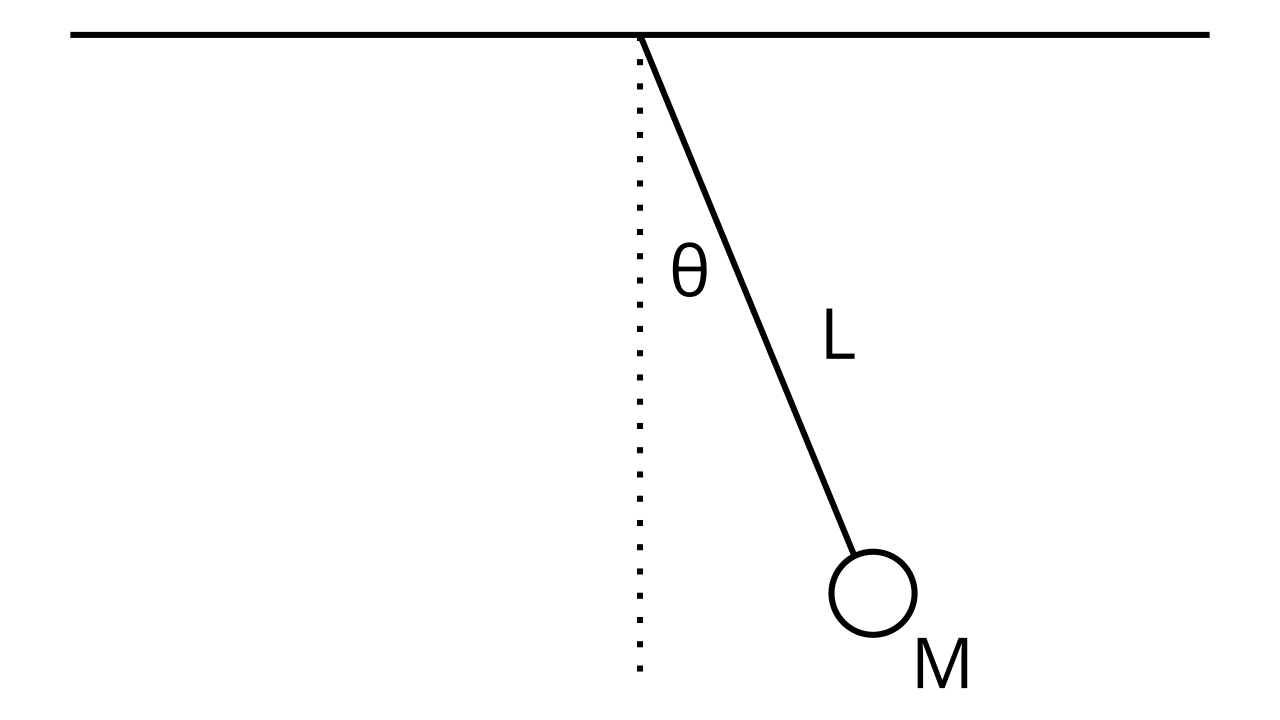
For the single pendulum problem, we first find the equations \(x(t)\) and \(y(t)\) given our coordinate system. Our coordinate system is based on the point \((0, 0)\) located at the point where the pendulum is attached to the ceiling. Using basic trigonometry, we find that:

\[ x(t) = \ell \sin \theta (t) \]

\[ y(t) = -\ell \cos \theta (t) \]

Where \(y(t)\) is negative because the pendulum is at a negative height relative to our origin. Using our expressions for \(x(t)\) and \(y(t)\), we want to find the expression for the kinetic energy \(K\). We know that:

\[ K = \frac{1}{2} mv^2 \]

And that:

\[ v = \sqrt{v_x^2 + v_y^2} = \sqrt{\left(\frac{dx}{dt}\right)^2 + \left(\frac{dy}{dt}\right)^2} \]

To do this, we solve for \(\frac{dx}{dt}\) and \(\frac{dy}{dt}\). This takes a bit of care, because we need to implicitly differentiate \(x(t)\) and \(y(t)\) with respect to \(t\), where:

\[ \frac{dx}{dt} = \frac{dx}{d\theta} \frac{d\theta}{dt} \]

\[ \frac{dy}{dt} = \frac{dy}{d\theta} \frac{d\theta}{dt} \]

Implicitly differentiating, we have:

\[ v_x = \frac{dx}{dt} = \ell \cos \theta \frac{d\theta}{dt} \]

\[ v_y = \frac{dy}{dt} = \ell \sin \theta \frac{d\theta}{dt} \]

Now, we plug our values for \(v_x\) and \(v_y\) into the kinetic energy equation, which gives us:

\[ K = \frac{1}{2} m \left(\ell^2 \cos^2 \theta \frac{d\theta}{dt} + \ell^2 \sin^2 \theta \frac{d\theta}{dt}\right) \]

If we do a little simplification by factoring and remembering that \(\cos^2 \theta + \sin^2 \theta = 1\), we get:

\[ K = \frac{1}{2} m \ell^2 \left(\frac{d\theta}{dt}\right)^2 \]

Now we find the potential energy. Remember that close to Earth, the potential energy is determined by and only by the vertical distance between the origin (which is the reference height of zero) and the measured point. This means that:

\[ U = mgh \]

The height in this case is negative (because it’s below the origin) and we’re only taking the vertical component of the height (hence \(\cos \theta\)) so:

\[ U = -mg \cos \theta \ell \]

Putting it all together, our Lagrangian is:

\[ \mathcal{L} = \frac{1}{2} m \ell^2 \left(\frac{d\theta}{dt}\right)^2 + mg \cos \theta \ell \]

Here, our coordinates are determined in terms of the angle \(\theta\) only, so the Euler-Lagrange equations take the form:

\[ \frac{d}{dt} \frac{\partial \mathcal{L}}{\partial \dot \theta} - \frac{\partial \mathcal{L}}{\partial \theta} = 0 \]

If we plug this into the Euler-Lagrange equation, we get:

\[ m \frac{d^2 \theta}{dt^2} \ell^2 + mg \sin \theta \ell = 0 \]

We can rewrite this as:

\[ m \frac{d^2 \theta}{dt^2} \ell^2 = - mg \sin \theta \ell \]

And cancel out the common factors to yield:

\[ \frac{d^2 \theta}{dt^2} = - \frac{g}{\ell} \sin \theta \]

We have arrived at our answer. This is the differential equation of the simple pendulum. Note that while this equation is impossible to solve analytically directly, we can use the small-angle approximation of \(\sin \theta \approx \theta\) to get:

\[ \frac{d^2 \theta}{dt^2} = -\frac{g}{\ell} \theta \]

Of which the solution is:

\[ \theta(t) = \theta_{max} \sin \left(\sqrt{\frac{g}{\ell}}t + \phi_0 \right) \]

Using Lagrangian mechanics to solve the orbit equation

We want to derive the orbit of Earth around the Sun. To do so, we again first derive the expressions for \(x(t)\) and \(y(t)\) in terms of the solar-earth system:

\[ x(t) = r(t) \cos \theta(t) \]

\[ y(t) = r(t) \sin \theta(t) \]

Differentiating both (and remembering to use the product rule), we find that:

\[ v_x(t) = \cos \theta(t) \frac{dr}{dt} - r(t) \sin \theta (t) \frac{d\theta}{dt} \]

\[ v_y(t) = \sin \theta(t) \frac{dr}{dt} + r(t) \cos \theta \frac{d\theta}{dt} \]

Which we can use to find the kinetic energy (after lots of algebra and several passes at using the identity \(\sin^2 \theta + \cos^2 \theta = 1\)):

\[ K = \frac{1}{2} m \left[\left(\frac{dr}{dt}\right)^2 + r^2 \left(\frac{d\theta}{dt}\right)^2\right] \]

The potential energy is given by \(U = -\frac{GMm}{r}\), so the Lagrangian is:

\[ \mathcal{L} = \frac{1}{2} m (\dot r^2 + r^2 \dot \theta^2) + \frac{GMm}{r} \]

Applying the Euler-Lagrange equations to each coordinate, \(r\) and \(\theta\), present in the Lagrangian, we have:

\[ \frac{d}{dt} \frac{\partial \mathcal{L}}{\partial \dot r} - \frac{\partial \mathcal{L}}{\partial r} = 0 \]

\[ \frac{d}{dt} \frac{\partial \mathcal{L}}{\partial \dot \theta} - \frac{\partial \mathcal{L}}{\partial \theta} = 0 \]

Solving both equations yields the equations of motion for the Earth:

\[ \frac{d^2 r}{dt^2} = r \left(\frac{d\theta}{dt}\right)^2 - \frac{GM}{r^2} \]

\[ \frac{d^2 \theta}{dt^2} = - \frac{2}{r} \frac{dr}{dt} \frac{d\theta}{dt} \]

These can be solved analytically, but for the sake of simplicity here they will be solved using a numerical differential equation solver:

import matplotlib.pyplot as plt
import numpy as np
from scipy.integrate import solve_ivp

def newtonian_d_dt(t, X, G=6.67e-11, M=2e30):
    r, theta, u, v = X
    dr_dt = u
    dtheta_dt = v
    du_dt = r * v ** 2 -(G * M) / (r ** 2) 
    dv_dt = -(2 * u * v) / r
    return dr_dt, dtheta_dt, du_dt, dv_dt

r0 = 1.5e11
theta0 = np.pi/2
u0 = 0
v0 = 1.99e-7 # 2pi / 365 days
newtonian_initial = [r0, theta0, u0, v0]

tmax = 365 * 24 * 60 * 60 # 1 year
samples = 5000
t = np.linspace(0, tmax, samples)
newtonian = solve_ivp(newtonian_d_dt, (0, tmax), y0=newtonian_initial, dense_output=True)
sol = newtonian.sol(t)

fig = plt.figure()
ax = plt.axes()

r = sol[0]
theta = sol[1]

# Convert from polar to cartesian
x1 = r * np.cos(theta)
y1 = r * np.sin(theta)

ax.plot(x1, y1)
ax.set_title('Plot of Newtonian orbit')
plt.show()

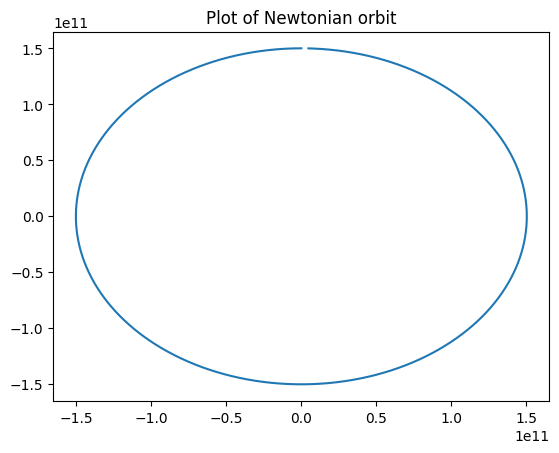
As it can be seen, the orbit is a ellipse, and we have arrived at this result using Lagrangian mechanics!

Using Lagrangians to solve the double pendulum problem

We will now tackle a problem that would be very difficult to solve using Newton’s laws, but much easier with Lagrangian mechanics. Here we have a system as follows:

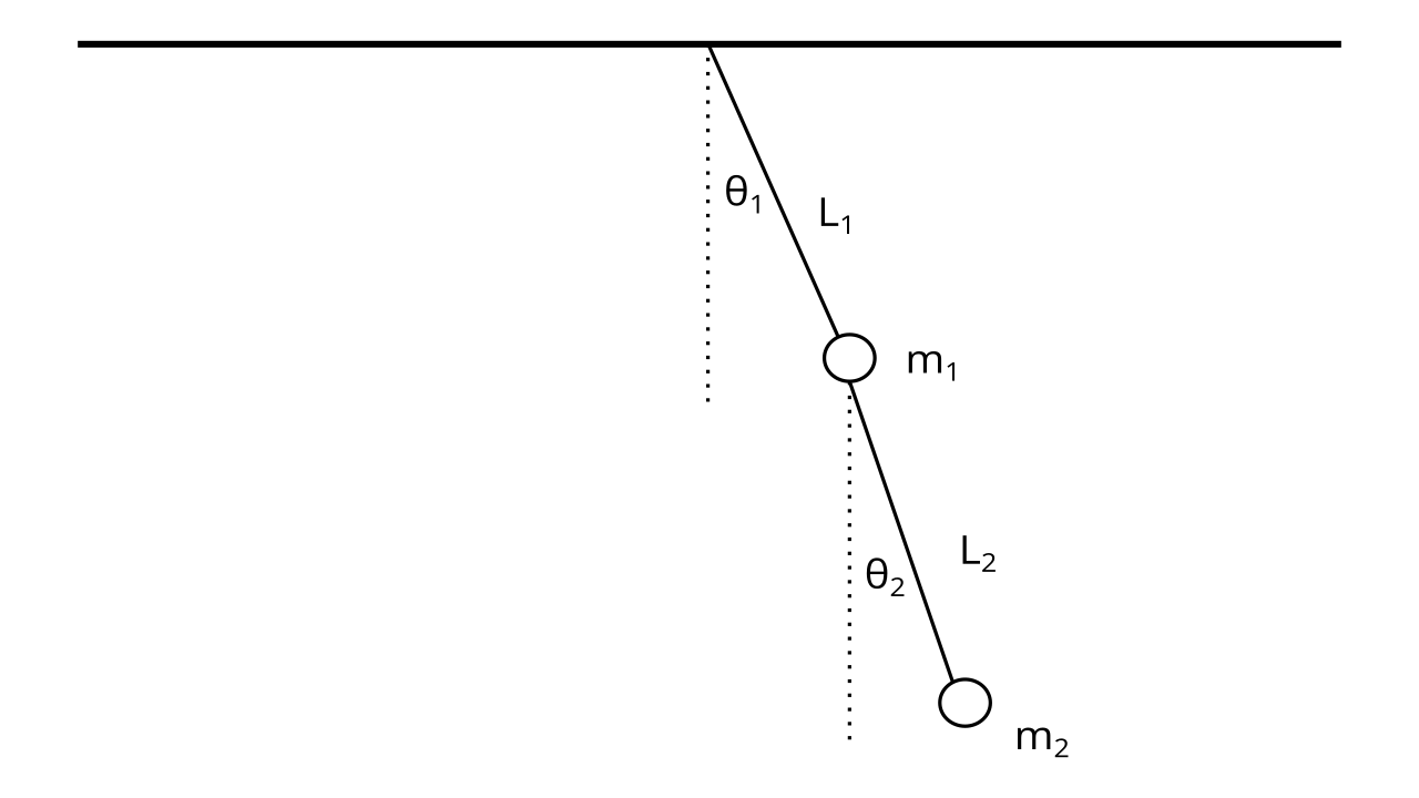
Here, the notable difference is that we have a system as opposed to a single object, and we need to find the kinetic and potential energies of the entire system. To do this, we divide the kinetic and potential energies into two parts:

\[ K = K_1 + K_2 \]

\[ U = U_1 + U_2 \]

Where \(K_1\) and \(K_2\) are respectively the kinetic energies of the first pendulum mass and second pendulum mass, and likewise with \(U_1\) and \(U_2\) and their potential energies.

We will first derive the kinetic energies, because they are harder :( As we know, we first setup a coordinate system where the point \((0, 0)\) is centered on the point the double pendulum is attached to the ceiling. Then, we write the position functions of the first pendulum:

\[ x_1(t) = \ell_1 \sin \theta_1 (t) \]

\[ y_1(t) = -\ell_1 \cos \theta_1 (t) \]

We figure these out from basic trigonometry and the fact that \(y_1(t)\) is negative, as it is below the origin. We then take the derivatives to find the \(x\) and \(y\) components of the velocity:

\[ \frac{dx_1}{dt} = \ell_1 \cos \theta_1 (t) \frac{d\theta_1}{dt} \]

\[ \frac{dy_1}{dt} = \ell_1 \sin \theta_1 (t) \frac{d\theta_1}{dt} \]

Using this, we can find \(K_1\):

\[ K_1 = \frac{1}{2} m_1 \left(\dot x_1^2 + \dot y_1^2\right) \]

\[ K_1 = \frac{1}{2} m_1 \left[ \left(\ell_1 \cos \theta_1 (t) \frac{d\theta_1}{dt} \right)^2 + \left(\ell_1 \sin \theta_1 (t) \frac{d\theta_1}{dt}\right)^2 \right] \]

Using the trig identity \(\sin^2 \theta + \cos^2 \theta = 1\), this is trivial to simplify into:

\[ K_1 = \frac{1}{2} m_1 \ell_1^2 \left(\frac{d\theta}{dt}\right)^2 \]

Then, we write the position functions of the second pendulum:

\[ x_2 (t) = x_1(t) + \ell_2 \sin \theta_2 (t) \]

\[ y_2 (t) = y_1(t) + (- \ell_2 \cos \theta_2 (t)) \]

Here, we add the \(x\) and \(y\) displacement of the second pendulum with the \(x\) and \(y\) displacement of the first to find the total displacement from the origin, because remember, we’re using the same coordinate system for both pendulums. If we sub in the values of \(x_1(t)\) and \(y_1(t)\), we have:

\[ x_2 (t) = \ell_1 \sin \theta_1 (t) + \ell_2 \sin \theta_2 (t) \]

\[ y_2 (t) = - \ell_1 \cos \theta_1 (t) - \ell_2 \cos \theta_2 (t)) \]

We compute their derivatives:

\[ \frac{dx_2}{dt} = \ell_1 \cos \theta_1 (t) \frac{d\theta_1}{dt} + \ell_2 \cos \theta_2(t) \frac{d\theta_2}{dt} \]

\[ \frac{dy_2}{dt} = \ell_1 \sin \theta_1(t) \frac{d\theta_1}{dt} + \ell_2 \sin \theta_2(t) \frac{d\theta_2}{dt} \]

And then plug them into the kinetic energy formula to find:

\[ K_2 = \frac{1}{2} m_2 \left[ \left(\ell_1 \cos \theta_1 (t) \frac{d\theta_1}{dt} + \ell_2 \cos \theta_2(t) \frac{d\theta_2}{dt}\right)^2 + \left(\ell_1 \sin \theta_1(t) \frac{d\theta_1}{dt} + \ell_2 \sin \theta_2(t) \frac{d\theta_2}{dt}\right)^2 \right] \]

Expanding that out, and using \(\sin^2 \theta + \cos^2 \theta = 1\) to simplify, we have:

\[ K_2 = \frac{1}{2} m_2 \left[ \ell_1^2 \left(\frac{d\theta_1}{dt}\right)^2 + 2\ell_1 \ell_2 \frac{d\theta_1}{dt} \frac{d\theta_2}{dt} (\cos \theta_1 \cos \theta_2 + \sin \theta_2 \sin \theta_2) + \ell_2^2 \left(\frac{d\theta_2}{dt}\right)^2 \right] \]

Here, we can use the identity \(\cos x \cos y + \sin x \sin y = \cos (x - y)\) to simplify to:

\[ K_2 = \frac{1}{2} m_2 \left[ \ell_1^2 \left(\frac{d\theta_1}{dt}\right)^2 + 2\ell_1 \ell_2 \frac{d\theta_1}{dt} \frac{d\theta_2}{dt} \cos (\theta_1 - \theta_2) + \ell_2^2 \left(\frac{d\theta_2}{dt}\right)^2 \right] \]

Now, combining the two kinetic energies together, we end up with:

\[ K = \frac{1}{2} m_1 \ell_1^2 \left(\frac{d\theta}{dt}\right)^2 + \frac{1}{2} m_2 \left[ \ell_1^2 \left(\frac{d\theta_1}{dt}\right)^2 + 2\ell_1 \ell_2 \frac{d\theta_1}{dt} \frac{d\theta_2}{dt} \cos (\theta_1 - \theta_2) + \ell_2^2 \left(\frac{d\theta_2}{dt}\right)^2 \right] \]

We use a similar approach for the potential energies - we add the potential energy of the first pendulum and the second to find the total system’s potential energy:

\[ U = U_1 + U_2 \]

\[ U = m_1 g (-\ell_1 \cos \theta_1 (t) ) + m_2 g (-\ell_1 \cos \theta_1(t) - \ell_2 \cos \theta_2(t)) \]

After factoring, we have:

\[ U = -(m_1 + m_2) g \ell_1 \cos \theta_1(t) - m_2 g \ell_2 \cos \theta_2 (t) \]

Using \(\mathcal{L} = K - U\), we substitute into the two Euler-Lagrange equations (one for \(\theta_1\) and one for \(\theta_2\)):

\[ \frac{d}{dt} \frac{\partial \mathcal{L}}{\partial \dot \theta_1} - \frac{\partial \mathcal{L}}{\partial \theta_2} = 0 \]

\[ \frac{d}{dt} \frac{\partial \mathcal{L}}{\partial \dot \theta_1} - \frac{\partial \mathcal{L}}{\partial \theta_2} = 0 \]

With the Lagrangian:

\[ \mathcal{L} = \frac{1}{2} m_1 \ell_1^2 \left(\frac{d\theta}{dt}\right)^2 + \frac{1}{2} m_2 \left[ \ell_1^2 \left(\frac{d\theta_1}{dt}\right)^2 + 2\ell_1 \ell_2 \frac{d\theta_1}{dt} \frac{d\theta_2}{dt} \cos (\theta_1 - \theta_2) + \ell_2^2 \left(\frac{d\theta_2}{dt}\right)^2 \right] + (m_1 + m_2) g \ell_1 \cos \theta_1(t) + m_2 g \ell_2 \cos \theta_2 (t) \]

To find the equations of motion (source):

\[ (m_1 + m_2) l_1 \ddot{\theta}_1 + m_2 l_2 \ddot{\theta}_2 \cos(\theta_1 - \theta_2) + m_2 l_2 \dot{\theta}_2^2\sin(\theta_1 - \theta_2) + (m_1 + m_2) g \sin\theta_1 = 0 \]

\[ l_2 \ddot{\theta}_2 + l_1 \ddot{\theta}_1 \cos(\theta_1 - \theta_2) - l_1 \dot{\theta}_1^2 \sin(\theta_1 - \theta_2) + g \sin\theta_2 = 0 \]

These equations are completely unsolvable analytically, but they can be solved numerically to yield the position of a double pendulum with time.

Langrangian to Newtonian mechanics

Let’s see how we can recover Newton’s 2nd law from the Euler-Lagrange equation. Remember that the equation (in the case of one-dimenional motion along the \(x\) axis) is given by:

\[ \frac{d}{dt}\frac{\partial \mathcal{L}}{\partial \dot x} = \frac{\partial \mathcal{L}}{\partial x} \]

And remember that the Lagrangian is given by:

\[ \mathcal{L} = \frac{1}{2} m \dot x^2 - U(x) \]

Applying the Euler-Lagrange equations to the general Lagrangian, we get:

\[ m \ddot x = -\frac{dU}{dx} \]

Recalling that \(F = -\frac{dU}{dx}\) and \(\ddot x = a\), we have recovered Newton’s 2nd law!

\[ F = ma \]

We can even use Lagrangian mechanics on simple problems and check that it matches with Newtonian mechanics. Let’s do our freefall example from earlier. With \(K = \frac{1}{2} m \dot y^2\) and \(U = mgy\), we use the Euler-Lagrange equations to find:

\[ m \frac{d^2 y}{dt^2} = - mg \]

Which we can simplify to:

\[ a_y = -g \]

Which reproduces the Newtonian result!

Hamiltonian mechanics

Noether’s theorem

Field Lagrangians

Besides working with particles and their trajectories, we are also often interested in fields in physics, such as the electromagnetic or gravitational fields. To find the differential equations that describe these fields, we need an Euler-Lagrange equation for fields rather than particles.

Let us consider a generic field \(\varphi(\mathbf{r}, t)\). For reasons that will be elaborated in more detailed in the special and general relativity sections (we will give a rough outline for why in a note further down this section), it is conventional to group the space and time components in one vector \(\mathbf{X}\) which has four components, one of time and three of space, and where \(c\) is the speed of light:

\[\begin{split} \mathbf{X} = (ct, \mathbf{r}) = \begin{bmatrix} ct \\ x \\ y \\ z \end{bmatrix} \end{split}\]

It is also convention to group the time derivative and gradient operators together, which we call the four-gradient and denote \(\partial_\mathbf{X}\):

\[ \partial_\mathbf{X} = \left(-\dfrac{1}{c}, \nabla\right) = \left\langle-\dfrac{1}{c}, \dfrac{\partial}{\partial x}, \dfrac{\partial}{\partial y}, \dfrac{\partial}{\partial z}\right\rangle \]

Note

Note for the advanced reader In special and general relativity, we call \(\mathbf{X}\) the four-position and we write it in tensor notation as \(x^\mu\), and we call \(\partial_\mathbf{X}\) the four-gradient and we write it similarly in tensor notation as \(\partial_\mu\). The reason we need these four-component vectors (and vector derivatives) is that in the theories of relativity, four-dimensional spacetime becomes of fundamental importance whereas space and time are reduced to perspective-dependent aspects of spacetime.

We will cover more on tensors in this chapter, but knowing tensors is not required for our (rough) treatment of Lagrangians in field theory. We will proceed with simply the four-position and four-gradient written in vector form.

With these new vectors we may write the field as \(\varphi(\mathbf{X})\). The action for the field is given by:

\[ S[\varphi, \partial_\mathbf{X} \varphi, \mathbf{X}] = \int_\Omega \mathcal{L(\varphi, \partial_\mathbf{X}\varphi, \mathbf{X})} d^4 x \]

Where \(\mathcal{L}\) is our field Lagrangian, \(d^4 x = dVdt\) is an infinitesimal portion of space and time, and \(\Omega\) is the domain of all space and all times. We will not repeat the full derivation of the Euler-Lagrange equation, but the steps are very similar to what we have already seen with the single-object Lagrangian case. The result is the Euler-Lagrange equation for fields, which takes the form:

\[ \dfrac{\partial \mathcal{L}}{\partial \varphi} - \dfrac{\partial}{\partial\mathbf{X}} \left(\dfrac{\partial \mathcal{L}}{\partial(\partial_\mathbf{X} \varphi)}\right) = 0 \]

Lagrangians to the stars

Note

This section is optional and discusses advanced physics, so by all means read on if interested, but otherwise feel free to skip this part!

The Lagrangian formulation of classical mechanics is so powerful, precisely because it relies on a differential equation that can be generalized. Beyond classical mechanics, the Lagrangian isn’t always necessarily \(\mathcal{L} = K - U\), but the Euler-Lagrange equations still hold true, and so does the principle of stationary action. Thus, a theory - including those that involve fields - can be written as a Lagrangian, as the Euler-Lagrange equations yield the equations of motion for each theory, on which the rest of the theory is built on! This is the reason behind learning Lagrangian mechanics.

We will end with one final thought - one of the most successful theories in all of physics, the Standard model of particle physics (which is a quantum field theory), is encapsulated in one compact Lagrangian:

\[ \mathcal{L}_\mathrm{SM} = -\frac{1}{4} F_{\mu \nu} F^{\mu \nu} + i \overline \psi \gamma_\beta D^\beta + h.c. + \psi_i y_{ij} \psi_j \phi + h.c. + |D_\mu \phi |^2 - V(\phi) \]

And one of the most mathematically beautiful theories, in fact one we will see very soon, General Relativity (which is a classical field theory for gravity), is described in another compact Lagrangian:

\[ \mathcal{L}_\mathrm{GR} = \frac{1}{2\kappa} R \sqrt{-g} + \mathcal{L}_\mathrm{matter} \]

Who knew that Lagrangians could take us deep into the hearts of atoms, and to the furthest stars…? :)