Quantum mechanics

“When you change the way you look at things, the things you look at change.”

Max Plank

Up to this point, we’ve explored physics that obeyed the principles of predictability and certainty. We took it for granted that particles moved on definite paths, that if we knew everything about the system we could predict everything about how it would evolve. All of those assumptions completely break down in quantum mechanics, when we take a look at the world near the scale of atoms. We’ll explore this fascinating new world - and in time, hopefully realize that, as Sean Carroll said, “the quantum world is not spooky or incomprehensible - it’s just way different”.

from matplotlib import cm
import matplotlib.pyplot as plt
import numpy as np

%matplotlib inline
plt.rcParams["font.family"] = "serif"
plt.rcParams['mathtext.fontset'] = 'stix'

Quantization and wavefunctions

When we speak of observable properties of a macroscopic object, such as its speed, momentum, and energy, we expect that these properties can take on any value. For instance, we can have a speed of 5.34 m/s, or 100,000 m/s, or 0.0015 m/s. These are called continuous properties.

But in the quantum world, certain properties of microscopic particles can only take certain values - specifically, values that are a multiple of some indivisible unit value. One way to think about it is to imagine you have several basketballs - it would make sense to have 0 basketballs, or 50 basketballs, or 12 basketballs, but it wouldn’t make sense to have \(\pi\) basketballs or 1.513 basketballs. The indivisible unit, in our case, is one basketball, and in quantum mechanics we call the unit a quantum (plural quanta). For example, the quantum of charge is the elementary charge constant \(e = 1.602 \times 10^{-19}\) Coulombs, which is exactly the charge of a single electron (ignoring the sign). This means that you can only have a charge of \(2e\) or \(5e\) or \(17e\), never \(1.352e\). We call properties that are composed of quanta quantized.

Energy is important, because it was Einstein who first discovered that the energy of light is quantized, and in particular that the quantum of light energy is given by:

\[ E_p = hf \]

where \(h\) is Plank’s constant, approximately \(6.626 \times 10^{−34}\), and \(f\) is the frequency of the wave - this is a result we will manually derive later. According to Einstein’s formula, this means that if you measure the energy of any light, it must be \(0E_p\) or \(1E_p\) or \(5E_p\) or \(1000E_p\), not \(1.5E_p\). Light can’t just take any energy it wants; the energy must strictly be \(N\cdot E_p\), where \(N\) is the number of photons in the measured light.

Einstein recognized that the quantization of light isn’t just a mathematical rule of integer multiples, but that quanta of light are actually the energy carried by physical particles that we call photons. But isn’t light a wave? Wasn’t that what Maxwell’s equations said? Physicists later recognized that Maxwell’s equations were incomplete - at a certain limit for smaller and smaller particles, they no longer offer a full description of electromagnetism.

More strange observations followed the discovery of light quanta (photons) and the recognition that electrons were the quantum of electric charge. Classically, electrons were modelled as (point) particles, with exact physical properties. But if an electron is a particle, why can’t we just measure its observable properties (such as position) and know how it behaves? Through experimentation, scientists tried, and failed, to do exactly this. They concluded that quantum particles cannot be found exactly. We can only measure probabilities by using a wavefunction that describes the state of a quantum system. The wavefunction is oftentimes a complex function, and has no direct physical meaning (which makes sense; all physical quantities are real numbers, not complex numbers!) However, it turns out that if you integrate the square of the wavefunction, you find the probability of a particle being at a particular position, which we write:

\[ P(x) = \int |\Psi(x, t)^2 | dx \]

Note

We will show later why \(P(x)\) does not have a dependence on time, even though \(\Psi(x, t)\) is a function of both space and time.

Note that we can generalize this to multiple dimensions:

\[ P(\mathbf{r}) = \int | \Psi(\mathbf{r}, t)^2 | \, dx \, dy \, dz \]

where \(\mathbf{r} = (x, y, z)\) is a shorthand for the three spatial coordinates. As an electron (or any other quantum particle) has to be somewhere, integrating over all space gives a probability of 1, that is, 100% probability of being at some point in space:

\[ \int_{-\infty}^\infty | \Psi(\mathbf{r}, t)^2 |~dx~dy~dz = 1 \]

Note

We typically use an uppercase \(\Psi\) for time-dependent wavefunctions and a lowercase \(\psi\) for time-independent wavefunctions.

The Schrödinger equation

If quantum systems are fundamentally probabilistic in nature, one may think that predicting any physical properties of them would be near-impossible. Fortunately, this is not the case. In fact, there exists a partial differential equation that can be solved to find the wavefunction \(\Psi(\mathbf{r}, t)\) for a single quantum particle: the Schrödinger equation. It is given by:

\[ i \hbar \frac{\partial \Psi}{\partial t} = \left(-\frac{\hbar^2}{2m} \nabla^2 + V(\mathbf{r}, t) \right) \Psi \]

Where \(\hbar = h/2\pi\) is Planck’s reduced constant, \(m\) is the mass of the particle, \(V\) is the potential energy of the particle, and \(i\) is the imaginary unit. Note that this expression for the Schrödinger equation applies to a single particle, not a system of particles; we will cover the multi-particle Schrödinger equation later.

Solving the Schrödinger equation yields the wavefunction, which can then be used to find the probability of a particle being at a certain position. As another stroke of luck, we find that when the potential \(V\) only depends on position, that is, \(V = V(\mathbf{r})\), then the Schrödinger equation becomes a separable linear differential equation.

This means that we have two (main) techniques for solving the Schrödinger equation by hand, based on the techniques we saw previously when we looked at how to solve PDEs in the differential equations section in the first chapter. We can either use the “method of inspired guessing” or the proper separation of variables technique. And we will cover both here.

Solving by inspired guessing

To solve the Schrödinger equation by inspired guessing, we first note that this approach only works when \(V(\mathbf{r}) = 0\). In addition, while we can use this technique in three dimensions, we will focus on the easier 1-dimensional case to start. The Schrödinger equation for \(V(\mathbf{r}) = 0\) (which is the case for a free particle unconstrained by any potential) becomes:

\[ i \hbar \frac{\partial \Psi}{\partial t} = -\frac{\hbar^2}{2m} \dfrac{\partial^2 \Psi}{\partial x^2} \]

Note that the Schrödinger equation looks quite similar to the heat equation that we studied earlier in the section on differential equations. Remember that the heat equation had solutions of sinusoids in space multipled with exponential solutions in time, so we would expect that the solutions to the Schrödinger equation would be at least somewhat similar. However, since the Schrödinger equation describes a complex-valued wavefunction instead of a real-valued heat distribution, we would expect complex-valued sinusoids. Recall that by Euler’s formula, we have \(e^{i\phi} = \cos \phi + i \sin \phi\) - therefore, we could make an educated guess that the spatial portion of the wavefunction would be a complex exponential with the form:

\[ \psi_x = e^{i k x} \]

where \(k\) is some constant factor to get the units right (remember that transcendental functions like \(e^x\) can only take dimensionless values in their argument). Now, recalling that the heat equation had exponential solutions in time, we would expect a complex exponential in time (since again, the Schrödinger describes a complex-valued wavefunction). In addition, recalling that the heat equation’s solutions in time were decaying exponentials, we would presume that the argument to the complex exponential would have a negative sign, with some constant factor to get the units right (which we’ll call \(\omega\)). So we could make the following guess:

\[ \psi_t = e^{-i \omega t} \]

Finally, recalling that a solution to the heat equation was formed by multiplying its spatial and temporal solution components, we can do the same to have:

\[ \Psi(x, t) = \psi_x \psi_t = e^{ikx} e^{-i\omega t} = e^{i(k x -\omega t)} \]

This is a plane wave that is a particular solution to the Schrödinger equation, and we can indeed verify it is correct by substituting it back into the Schrödinger equation. First, we compute the derivatives:

\[\begin{split} \begin{align*} \dfrac{\partial \Psi}{\partial t} &= \dfrac{\partial}{\partial t} e^{i(k x - \omega t)} = -i \omega e^{i (k x - \omega t)} \\ \dfrac{\partial \Psi}{\partial x} &= \dfrac{\partial}{\partial x} e^{i(k x- \omega t)} = i k e^{i(kx - \omega t)} \\ \dfrac{\partial^2\Psi}{\partial x^2} &= \dfrac{\partial}{\partial x} \left(\dfrac{\partial \Psi}{\partial x}\right) = \dfrac{\partial}{\partial x} ik e^{i(kx - \omega t)} = -k^2 e^{i (k x - \omega t)} \\ \end{align*} \end{split}\]

Then, we plug these derivatives back into the Schrodinger equation:

\[\begin{split} \begin{align*} i \hbar \frac{\partial \Psi}{\partial t} &= -\frac{\hbar^2}{2m} \dfrac{\partial^2 \Psi}{\partial x^2} \Rightarrow \\ i\hbar(-i\omega e^{i (k x - \omega t)}) &= -\dfrac{\hbar^2}{2m}(-k^2) e^{i (k x - \omega t)} \\ \hbar \omega e^{i (kx - \omega t)} &= \dfrac{\hbar^2 k^2}{2m} e^{i(kx - \omega t)} \\ \hbar\omega &= \dfrac{\hbar^2 k^2}{2m} \end{align*} \end{split}\]

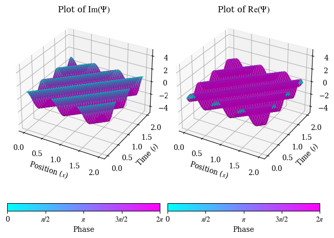
In which we find that the Schrödinger equation is indeed satisfied, as long as \(\hbar \omega = \dfrac{\hbar^2 k^2}{2m}\). A Python-generated plot of a plane wave is shown below (the code is unfortunately rather lengthy):

# Data for plotting
tmin, tmax = 0, 2
xmin, xmax = 0, 2
samples = 2000

t = np.arange(tmin, tmax, (xmax - xmin)/samples)
x = np.arange(xmin, xmax, (tmax - tmin)/samples)

# wavelengths in spatial domain
space_cyles = 3
# periods in temporal domain
time_cycles = 3

wavelength = (xmax - xmin) / space_cyles
period = (tmax - tmin) / time_cycles
freq = 1/period
k = 2 * np.pi / wavelength
omega = 2 * np.pi * freq

T, X = np.meshgrid(t, x)
phase = k*X - omega*T
psi = np.exp(1j*phase) # j is imaginary unit in Python
magn = np.abs(psi)

def wavefunction_component_ax3d(ax, x=x, t=t, X=X, T=T, phase=phase, ptype="real"):
    # create colormap based on phase
    phase_0_to_2pi = phase % (2*np.pi) # to rescale phase to [0, 2pi]
    cmap = cm.cool(phase_0_to_2pi/2)
    # distinguish between real/imaginary components via ptype arg
    if ptype == "imaginary":
        psi_label = r"$\text{Re}(\Psi)$"
        ax.plot_surface(X, T, np.imag(psi), linewidth=0,
                        facecolors=cmap)
    elif ptype == "real":
        psi_label = r"$\text{Im}(\Psi)$"
        ax.plot_surface(X, T, np.real(psi), linewidth=0,
                        facecolors=cmap)
    else:
        print("You didn't specify a ptype (real or imaginary)")
        return
    
    ax.set(title=r"Plot of " + psi_label)
    ax.set(xlabel=r"Position ($x$)", ylabel=r"Time ($t$)", zlabel=psi_label)
    ax.set(zlim=(-5, 5))
    ax.grid()
    return ax

def create_cbar(ax, x=x, t=t):
    # create colorbar
    phase_range = k*x - omega*t # as we need it 1-dimensional
    norm=plt.Normalize(float(np.min(phase_range)), float(np.max(phase_range)))
    sm = cm.ScalarMappable(norm=norm, cmap=cm.cool)
    sm.set_clim(0, 2*np.pi)
    cbar = plt.colorbar(sm, ax=ax, orientation="horizontal")
    cbar.set_ticks([0, np.pi/2, np.pi, 3*np.pi/2, 2*np.pi])
    cbar.set_ticklabels(["0", r"$\pi/2$", r"$\pi$", r"$3\pi/2$", r"$2\pi$"])
    cbar.set_label("Phase")

fig, (ax1, ax2) = plt.subplots(1, 2, subplot_kw={"projection": "3d"})
fig.tight_layout()

# add each of the graphs
wavefunction_component_ax3d(ax1, ptype="real")
wavefunction_component_ax3d(ax2, ptype="imaginary")

# colorbar
create_cbar(ax1)
create_cbar(ax2)

# plot results
plt.show()

Let us now find a physical interpretation of \(k\) and \(\omega\). We note by dimensional analysis, in SI units, \(k\) must have units of inverse meters. There is one quantity we know of that has inverse meters, from our study of electromagnetic waves - the wavenumber, where \(k = \dfrac{2\pi}{\lambda}\). This suggests that surprisingly, quantum particles have some sort of “wavelength”, a characteristic feature of a wave. This wavelength is called the de Broglie wavelength, and means that like waves, quantum particles can travel around obstacles, interefere and diffract, and even pass right through each other. This is why the Schrödinger equation is considered a wave equation, and as a result, quantum particles are not localized in space before measurement. Even more bizarrely, the de Broglie wavelength gives rise to an equation for a quantum particle’s momentum:

\[ p = \dfrac{h}{\lambda} = \hbar k \]

which means that a quantum particle can have momentum even if it does not have mass. Photons, for instance, are massless particles, yet they can exert momentum (radiation pressure) on objects.

Let us now return to the other constant factor, \(\omega\). By similar dimensional analysis, we note that \(\omega\) must have units of inverse seconds. This suggests some form of frequency. In fact, it is the angular frequency. Now, recall we previously derived that \(\hbar \omega = \dfrac{\hbar^2 k^2}{2m}\). Using the substitution that \(p = \hbar k\), we can rewrite this as:

\[ \hbar \omega = \dfrac{\hbar^2 k^2}{2m} = \dfrac{p^2}{2m} = \dfrac{(mv)^2}{2m} = \dfrac{1}{2} mv ^2= E \]

Using the special case of photons, we can justify why \(\omega\) must be the angular frequency. Recall that \(E = hf\) expresses the energy carried by a single photon. But we also know that \(E = \hbar \omega\) and \(\hbar = h/2\pi\). Therefore, equating all our expressions together, we have:

\[\begin{split} \begin{gather*} E = hf = \hbar \omega = \dfrac{h}{2\pi} \omega \\ h f = \dfrac{h}{2\pi }\omega \\ f = \dfrac{\omega}{2\pi} \Rightarrow \omega = 2\pi f \end{gather*} \end{split}\]

And therefore we have shown that \(\omega\) must be the angular frequency. Note that the formulas we found unintentionally while solving the Schrödinger equation, \(p = \hbar k\) and \(E = \hbar \omega\), show that there is a fundamental connection between momentum and \(k\) and similarly between energy and \(\omega\). This is, in fact, a relationship that will hold even when the Schrödinger equation itself becomes inaccurate in certain physical scenarios.

Now, there is one particular issue in our solution to the Schrödinger equation: it’s physically impossible. Recall that the normalization condition, which guarantees that a particle is at least somewhere in space, requires that:

\[ \int_{-\infty}^\infty |\Psi(x, t)^2 | dx = 1 \]

But if we attempt to integrate our plane-wave solution \(\Psi(x, t) = e^{i(kx - \omega t)}\) we will find that this condition is not satisfied:

\[\begin{split} \begin{align*} \int_{-\infty}^\infty |\Psi(x, t)^2 | dx &= \int_{-\infty}^\infty \Psi(x, t) \Psi^*(x, t)\, dx \\ &= \int_{-\infty}^\infty e^{i(kx - \omega t)} e^{-i(kx - \omega t)} dx \\ &= \int_{-\infty}^\infty d x \\ &= \infty \end{align*} \end{split}\]

Therefore, the particle would have infinite probability of being somewhere in space - nonsensical! However, it turns out that there is a way to make sense out of a plane-wave solution. If we instead take a sum of plane waves of different wavelengths (and therefore a unique \(k\) for each wave), then certain portions of each wave will cancel out with the others and certain portions will combine together - that is, the waves would interfere. Therefore, a solution in the form:

\[ \Psi(x, t) = \sum_n e^{i(k_nx - \omega t)} \]

does in fact have a finite probability of being somewhere in space. In the continuum limit where we sum over an infinite number of plane waves (and therefore an infinite number of different \(k\)’s) the sum becomes an integral, so we have:

\[ \Psi(x, t) = \dfrac{1}{\sqrt{2\pi}} \int_\infty^\infty A(k) e^{i(kx - \omega t)} d x \]

This is known as a wave packet solution for a free (quantum) particle and in fact is perfectly normalizable - the factor of \(\dfrac{1}{\sqrt{2\pi}}\) is needed to satisfy the normalization condition (i.e. that the total probability of the particle existing something in space is 100%). The function \(A(k)\) gives the distribution of \(k\) (and therefore the distribution of momenta) for \(\Psi(x, t)\). The exact form of \(A(k)\) is dependent on the physical scenario we are considering, but one very common choice of \(A(k)\) that is widely-applicable is the Gaussian:

\[ A(k) = \sqrt{\sigma}\left(\dfrac{2}{\pi}\right)^{1/4} e^{-\sigma^2 (k - k_0)^2} \]

For which \(\Psi(x, t)\) becomes, after evaluation of the integral:

\[ \psi(x, t) =\left( \dfrac{1}{2 \pi} \right)^{1 / 4} \dfrac{1}{\sqrt{\sigma}} e^{i k_0 x - \frac{x^2}{4 \sigma^2}} e^{-i \omega t} \]

Solving by separation of variables

Recall that since the Schrödinger equation is separable, we may use the technique of the separation of variables to make it solvable. To do so, we first assume a solution in the form \(\Psi(\mathbf{r}, t) = \psi(\mathbf{r}) T(t)\), where \(\psi(\mathbf{r})\) is the purely-spatial component, and \(T(t)\) is the purely-temporal (time) component. Then, we can take the derivatives to have:

\[\begin{split} \begin{align*} \dfrac{\partial \Psi}{\partial t}&= \dfrac{\partial}{\partial t}\psi(\mathbf{r}) T(t) = \dfrac{dT}{dt} \psi(\mathbf{r}) \\ \nabla \Psi &= \nabla [\psi(\mathbf{r}) T(t)] = T(t) \nabla \psi(\mathbf{r}) \\ \nabla^2 \Psi &= \nabla(\nabla [\psi(\mathbf{r}) T(t)]) = T(t) \nabla^2 \psi(\mathbf{r}) \\ \end{align*} \end{split}\]

Note

As \(T(t)\) depends on only one variable (\(t\)) the partial derivative becomes an ordinary derivative.

Plugging these back into the Schrödinger equation we have:

\[\begin{split} \begin{align*} i\hbar \dfrac{\partial}{\partial t} \Psi &= \left(-\dfrac{\hbar^2}{2m} \nabla^2 + V(\mathbf{r})\right) \Psi \\ i\hbar \dfrac{dT}{dt}\psi(\mathbf{r}) &= -\dfrac{\hbar^2}{2m} T(t) \nabla^2 \psi + V(\mathbf{r})\psi(\mathbf{r}) T(t) \end{align*} \end{split}\]

Dividing both sides by \(\psi(\mathbf{r})T(t)\) we have:

\[\begin{split} \begin{align*} \dfrac{1}{\psi(\mathbf{r})T(t)}i\hbar \dfrac{dT}{dt}\psi(\mathbf{r}) &= \dfrac{1}{\psi(\mathbf{r})T(t)} \left[-\dfrac{\hbar^2}{2m} T(t) \nabla^2 \psi + V(\mathbf{r})\psi(\mathbf{r}) T(t)\right] \\ \dfrac{i\hbar}{T(t)} \dfrac{dT}{dt} &=\dfrac{1}{\psi(\mathbf{r})} \left[-\dfrac{\hbar^2}{2m} \nabla^2 \psi + V(\mathbf{r})\psi(\mathbf{r}) \right] \end{align*} \end{split}\]

Remember that just as previously when we did separation of variables, the left and right-hand sides of the last equation are equal to a constant as two derivatives can only be equal in value if they are equal to a constant. We will call this constant \(E\), and by dimensional analysis we can find that this is indeed equal to the total energy of the particle (there is a more elegant argument for why we may interpret the separation constant \(E\) as the energy, that we will cover later). Thus, we are able to simplify the Schrödinger equation into two simpler equations, one only depend on space and one only dependent on time:

\[\begin{split} \begin{align*} \dfrac{i\hbar}{T(t)} \dfrac{dT}{dt} &=\dfrac{1}{\psi(\mathbf{r})} \left[-\dfrac{\hbar^2}{2m} \nabla^2 \psi + V(\mathbf{r})\psi(\mathbf{r}) \right] = E \\ \dfrac{i\hbar}{T(t)} \dfrac{dT}{dt} &= E \quad \Rightarrow \quad i\hbar \dfrac{dT}{dt} = E\,T(t) \\ \dfrac{1}{\psi(\mathbf{r})} &\left[-\dfrac{\hbar^2}{2m} \nabla^2 \psi + V(\mathbf{r})\psi(\mathbf{r}) \right] = E \\ &\Rightarrow -\dfrac{\hbar^2}{2m} \nabla^2 \psi + V(\mathbf{r})\psi(\mathbf{r}) = E \psi(\mathbf{r}) \end{align*} \end{split}\]

The differential equation in time, \(i\hbar \dfrac{dT}{dt} = E\,T(t)\), is an equation that we are experienced in solving. Its solution is a complex exponential:

\[ T(t) = e^{-iE t / \hbar} \]

Which we can verify by substituting by into the differential equation \(T(t)\). Note that as we found that \(E =\hbar \omega\), then we may rearrange to find that \(\frac{E}{\hbar} = \omega\), and thus it is also acceptable to write:

\[ T(t) = e^{-i\omega t} \]

Which is a form we will also use in the following sections. The differential equation in time, as we have seen, is straightforward to solve and yields a complex exponential as its solution.

The differential equation in space, however, has much richer and more complex solutions. In fact, this is the equation we primarily focus on when we say we are “solving the Schrödinger equation”. It is so crucial that it has its own name: the time-independent Schrödinger equation:

\[ -\dfrac{\hbar^2}{2m} \nabla^2 \psi + V(\mathbf{r})\psi(\mathbf{r}) = E \psi(\mathbf{r}) \]

The exact solution \(\psi(\mathbf{r})\) to the time-independent Schrödinger equation depends on the physics of the situation to analyze. After solving the time-independent Schrödinger equation, recalling that \(\Psi(\mathbf{r}, t) = \psi(\mathbf{r})T(t)\), we find that the time-dependent wavefunction is given by:

\[ \Psi(\mathbf{r}, t) = \psi(\mathbf{r}) e^{-iE t / \hbar} \]

But if \(\psi_1\) is a solution to the time-independent Schrödinger equation, then by linearly, so is \(\psi_2\), and so is \(\psi_3, \psi_4, \psi_5, \dots, \psi_n\), and each solution \(\psi_n\) has a corresponding energy \(E_n\). Therefore, the most general solution is found by summing over all \(\psi\), with constant-valued coefficients \(c_n\) for each \(\psi_n\):

\[ \Psi(\mathbf{r}, t) = \sum_n c_n\psi_n(\mathbf{r})T_n(t) = \sum_ic_n\psi_n(\mathbf{r}) e^{-iE_n t / \hbar} \]

This is not simply a mathematical trick; the physical significance of the general solution as a sum of individual solutions \(\psi_n\) is that each quantum system, which has a wavefunction \(\Psi(\mathbf{r}, t)\), is composed of states \(\psi_n\). The wavefunction is such that the system has some probabiliy \(P_n = |c_n|^2\) of being in the \(n\)th-state. The particle can be in any one of the states, but we can only predict probabilities it is in a particular state; we cannot predict which exact state it is in.

The theoretical approach to solving for the wavefunction, it seems, is not too hard: simply solve the time-independent Schrödinger equation for all the states \(\psi_n(\mathbf{r})\), add a time factor \(e^{-iE_n t/\hbar}\), and then write the general solution as a sum over all the states with appropriate coefficients \(c_n\), which we can find using the requirement that:

\[ \displaystyle \sum_n |c_n|^2 = |c_1|^2 + |c_2|^2 + |c_3|^2 + \dots + |c_n|^2 = 1 \]

However, the simplicty is deceptive; as with most differential equations, getting to an exact solution is not easy, and sometimes impossible. Thus, for real-life applications (where we cannot assume idealized theoretical systems), Schrödinger’s equation is usually solved numerically, using the finite difference method, the finite volume method, or the finite element method, which we will discuss later.

Observables, operators, and eigenvalue problems

Just like how we explored the quantization of energy for photons, other measurable quantities, such as the energy and momentum of quantum particles, can also be quantized. In fact, we just derived two cases of quantized quantities: \(E = \hbar \omega_0\) and \(p = \hbar k\). In the general case, we call measurable quantities observables in quantum mechanics. Observables have defined real values, but those values are discrete values, not continuous functions. Therefore, since observables are discrete numbers, then momentum, energy, and angular momentum, as well as other properties cannot be represented by functions, as functions have continuous outputs.

But we know of one different mathematical representation that can work to give discrete numbers - eigenfunctions and eigenvalues. Indeed, in quantum mechanics, any observable \(A\) has an associated operator \(\hat A\). The operator follows an eigenvalue equation, such that:

\[ \hat A \psi = a \psi \]

Here, \(\hat A\) is a linear operator acting on \(\psi\). The most common type of linear operator for eigenfunctions are derivative operators. For instance, the momentum operator (in one dimension) is given by:

\[ \hat p = -i\hbar \frac{\partial}{\partial x} \]

So if we wanted to find the measured value of the momentum \(p\), we would need to solve the eigenvalue equation:

\[ \hat p \psi = p \psi \]

By substitution of the explicit form of the momentum operator we have:

\[ -i\hbar \frac{\partial \psi}{\partial x} = p \psi \]

This is a differential equation with the solution \(\psi(x) = C_1 e^{ipx/\hbar}\). But you may think, that’s just a plane wave - which we know is unphysical! Indeed, that is true, but recalling our trick with the free particle, we may sum infinite numbers of plane waves together such that we have a normalizable solution, which becomes an integral in the continuous limit:

\[ \psi(x) = \dfrac{1}{\sqrt{2\pi\hbar}}\int_\infty^\infty B(p)e^{i p x} dp \]

Where \(B(p)\) is the distribution of momenta. This ensures that the observable - in this case, the measured value of momentum - stays a discrete number, rather than a continuous function, satisfying the eigenvalue equation for the momentum operator, while \(\psi(x)\) also satisfies normalizablity.

From the momentum operator, we may derive the kinetic energy operator. Recall that in classical mechanics, the kinetic energy is defined by \(K = \dfrac{1}{2} mv^2 = \dfrac{p^2}{2m}\). In an analogous fashion, in quantum mechanics, the kinetic energy can be found from the momentum operator by the same general formula:

\[ \hat K = \dfrac{\hat p^2}{2m} = \dfrac{\hat p \cdot \hat p}{2m} = \dfrac{\hbar^2}{2m} \dfrac{\partial^2}{\partial x^2} \]

What about the potential energy? Remember that the potential energy in classical physics does not depend on the velocity of a particle or time; it depends only on its position. Therefore, the potential energy operator remains unchanged in quantum mechanics, and we have:

\[ \hat V = V(x) \]

So, the eigenfunction-eigenvalue equations for kinetic energy and potential energy are given by:

\[\begin{split} \begin{align*} \hat K \psi &= -\frac{\hbar^2}{2m} \frac{\partial^2 \psi}{\partial x^2} = K \psi \\ \hat V \psi &= V(x) \psi \end{align*} \end{split}\]

But what about continuous distributions of momentum and energy, you may ask? Why does the potential energy operator, for instance, have a function rather than a discrete eigenvalue. The answer is that these distributions still have discrete and quantized eigenvalues, just infinitely many of them.

Now, let us take another look at the kinetic energy and potential energy operators:

\[\begin{split} \begin{align*} \hat K &= -\frac{\hbar^2}{2m} \frac{\partial^2}{\partial x^2} \\ \hat V &= V(x) \end{align*} \end{split}\]

But remember that the total energy, which is represented by the Hamiltonian operator, is given by:

\[ \hat H = -\frac{\hbar^2}{2m} \frac{\partial^2}{\partial x^2} + V(x) = \hat K + \hat V \]

This is simply the conservation of energy! Notice the energy operator is the sum of the kinetic energy operator and the potential energy. But since we have \((\hat K + \hat V)\psi = \hat H \psi\) for the operators, then we also have \((K + V)\psi = E\psi\) for the eigenvalues. Combining these together we get:

\[ \hat H \psi = E \psi \]

This is the time-independent Schrödinger equation. It offers a crucial insight into the nature of quantum systems: to find the possible states of a quantum system, we need to find the eigenfunctions of the Hamiltonian, and knowing the possible states also gives us the possible energies of the system (which are often quantized). This is a very important insight as it generalizes to more advanced quantum mechanics and the research that we do.

The uncertainty principle

Knowing more about a particular observable in general means that we know less about another observable. This is the uncertainy principle - when we express the uncertainty of position and momentum in terms of their standard deviations \(\sigma_x, \sigma_p\), then:

\[ \sigma_x \sigma_p \geq \frac{\hbar}{2} \]

To derive this, let’s consider the position and momentum operators. They are given respectively by:

\[ \hat x = x, \quad \hat p = -i\hbar \frac{\partial}{\partial x} \]

Now, it is important to recognize that these two operators do not commute - if we switch the order we apply these operations, we get different results. That is:

\[ \hat x \hat p \psi \neq \hat p \hat x \psi \]

We call the difference between applying these two operators in either order the commutator, denoted by square brackets:

\[ [\hat x, \hat p] = \hat x \hat p - \hat p \hat x \]

If we compute this commutator by substituting the operators in, we get:

\[ [\hat x, \hat p] = i \hbar \]

We can now make use of a theorem from statistics, which says that:

\[ \sigma_a \sigma_b \geq \frac{1}{2i} [\hat a, \hat b] \]

Plugging in our result for the commutator, we get the Heisenberg uncertainty principle:

\[ \sigma_x \sigma_p \geq \frac{\hbar}{2} \]

The Heisenberg uncertainty principle places further restrictions on the limits of observational and experimental precision, meaning that position and momentum cannot both be perfectly known. When measuring the position of the particle, the momentum is not known precisely as there is uncertainty in momentum, meaning that the particle’s momentum could be fluctuate within the bounds of the uncertainty; similarly, when measuring the momentum of a particle, the position is not known precisely as there is uncertainty in position, meaning that the particle’s position could be anywhere within the bounds of the uncertainty in position. Further, when position is perfectly known, the uncertainty in momentum is infinite, and so the momentum is not known at all! The same goes for momentum - when it is perfectly known, the uncertainty in position is infinite, meaning that the particle could be anywhere!