Numerical Simulations, Part 1#
In the previous chapter, we discussed the general ideas behind finite element analysis, and derived a weak form for the wave equation and its closely-related time-independent cousin, the Helmholtz equation. However, we did not discuss how to actually translate these ideas into code so that they can be solved by finite-element software. This is what we will cover in this section.
 1import numpy as np
 2import matplotlib.pyplot as plt
 3from numpy.linalg import norm
 4from findiff import FinDiff
 5from findiff.diff import Coef, Id
 6from findiff.pde import BoundaryConditions, PDE
 7import scipy.sparse as sparse
 8import scipy.optimize as optimize
 9from numpy.linalg import norm
10from random import randint
11from sklearn.preprocessing import StandardScaler
12from sklearn.neural_network import MLPRegressor
1%matplotlib inline
2# settings for professional output
3plt.rcParams["font.family"] = "serif"
4plt.rcParams["axes.grid"] = True
5plt.rcParams["mathtext.fontset"] = "stix" # use STIX fonts (install from https://www.stixfonts.org/)
6# optional - always output SVG (crisper graphics but often slow)
7# %config InlineBackend.figure_format = 'svg'
Finite element analysis#
Warning
This section is not yet complete. FENiCs code will be added here to demonstrate the finite element simulations at some point.
Scalar-valued validation test#
Up to this point, our results look correct. But do we know if they are? This is a tricky answer because most numerical problems - including the one we are analyzing - do not have analytical solutions. However, we can validate our finite-element results by comparing against another numerical solver. Specifically, we will compare our results to a solve using a different numerical technique - the finite difference method (FDM).
To simplify our analysis, we begin by working with the scalar variant of the Helmholtz equation, which is given by:
This is the exact same as the finite element formulation which we will keep for consistency. We wish to solve it via the finite difference method with a discrete Laplacian:
 1k = 3.0
 2# this has to be set to a low number or else the generated mesh
 3# might take up too much memory and crashing Python
 4squaren = 30
 5shape = (squaren, squaren)
 6
 7x = np.linspace(0, 1, squaren)
 8y = np.linspace(0, 1, squaren)
 9X, Y = np.meshgrid(x, y, indexing='ij')
10
11dx = 1 / squaren
12dy = 1 / squaren
13
14bc = BoundaryConditions(shape)
15bc
<findiff.pde.BoundaryConditions at 0x7fa83c884d40>
In our domain, we set a simple problem to solve, using the Dirichlet boundary conditions \(E \big|_{\partial \Omega} = \text{const.}\):
1bc[:, 0] = 3 # E(x, 0)
2bc[:, -1] = 10 # E(x, 1)
3bc[0, :] = 6 # E(0, y)
4bc[-1, :] = 1 # E(1, y)
We have two FDM solvers - a custom solver solve_Helmholtz_equation() and a wrapper for FinDiff’s own solver findiff_solve_Helmholtz_equation(), which are below.
For Project Elara researchers
Previously in testing there was a findiff “issue” with the construction of the operator \(\nabla^2 + k^2\). It would be preferable to just convert the stuff to a matrix to solve because it is still unknown whether Coef(k**2)*Id() is the correct way to construct it. But seems like now that it yielded the correct solution all along and the solution was just thought to be wrong.
1def findiff_solve(bc=bc, grid_shape=shape, k=k, dx=dx, dy=dy):
2    Helmholtz = FinDiff(0, dx, 2) + FinDiff(1, dy, 2) + Coef(k**2)*Id()
3    rhs = np.zeros(grid_shape)
4    pde = PDE(Helmholtz, rhs, bc)
5    return pde.solve()
1def create_Helmholtz_operator(dx, dy, grid_shape, k):
2    n, m = grid_shape
3    laplacian = FinDiff(0, dx, 2) + FinDiff(1, dy, 2)
4    ksquared = k**2 * sparse.eye(np.prod(grid_shape))
5    # reshape() automatically selects to whichever shape necessary
6    Helmholtz_mat = laplacian.matrix(grid_shape) + ksquared
7    return Helmholtz_mat
 1def solve_Helmholtz_equation(dx=dx, dy=dy, bc=bc, grid_shape=shape, k=k):
 2    Helmholtz = create_Helmholtz_operator(dx, dy, grid_shape, k)
 3    rhs = np.zeros(shape)
 4    f = rhs.reshape(-1, 1)
 5    # set boundary conditions
 6    # this code is copied over from
 7    # findiff's source code in findiff.pde.PDE.solve()
 8    nz = list(bc.row_inds())
 9    Helmholtz[nz, :] = bc.lhs[nz, :]
10    f[nz] = np.array(bc.rhs[nz].toarray()).reshape(-1, 1)
11    print("Solving (this may take some time)...")
12    solution = sparse.linalg.spsolve(Helmholtz, f).reshape(grid_shape)
13    print("Solving complete.")
14    return solution
 1def plot_E(E, X=X, Y=Y, label="Surface plot of solution data", rot=30):
 2    fig = plt.figure()
 3    ax = fig.add_subplot(projection='3d')
 4    ax.set_xlabel("$x$")
 5    ax.set_ylabel("$y$")
 6    ax.set_zlim(np.min(E), np.max(E))
 7    ax.view_init(30, rot)
 8    surf = ax.plot_surface(X, Y, E, cmap="coolwarm")
 9    fig.colorbar(surf, shrink=0.6)
10    if not label:
11        plt.title("Surface plot of solution data (v2)")
12    else:
13        plt.title(label)
14    plt.show()
1E = solve_Helmholtz_equation()
2E_findiff = findiff_solve()
Solving (this may take some time)...
Solving complete.
However, the solution is different in form to the typical mathematical (Cartesian) representation. This is because arrays are stored in (row, column) order, that is, \((y, x)\), as is standard for computers, and in addition to this their origin is located at the top-left, rather than the bottom-left as is used in Cartesian coordinates. So we must convert to the standard mathematical representation before displaying. This consists of transposing, then flipping the array along the columns axis.
 1def correct_axes(mat2d):
 2    return np.flip(mat2d.T, axis=0)
 3
 4def calibrate(x=X, y=Y):
 5    f = (y - 0.4)**2 # the asymmetrical test function for calibration
 6    plt.imshow(correct_axes(f), interpolation="none")
 7    plt.title(r"Calibration test")
 8    plt.grid(False)
 9    plt.colorbar()
10    plt.show()
1calibrate()
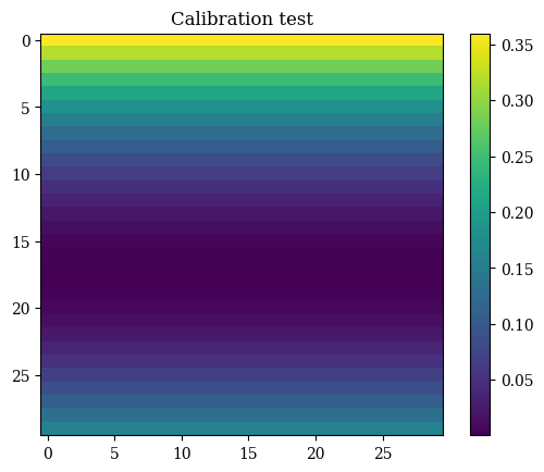
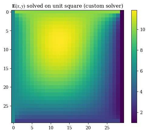
Performing the proper transformation to yield the correct representation for images, we can see the results below:
1plt.imshow(correct_axes(E), interpolation="none")
2plt.title(r"$\mathbf{E}(x, y)$ solved on unit square (custom solver)")
3plt.colorbar()
4plt.grid(False)
5plt.show()
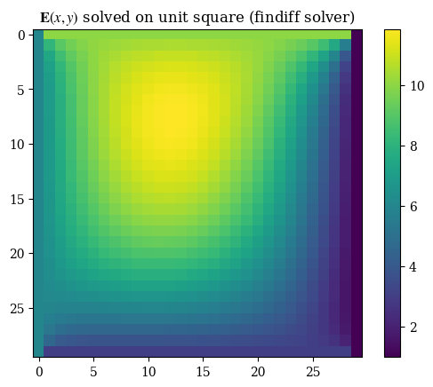
1plt.imshow(correct_axes(E_findiff), interpolation="none")
2plt.title(r"$\mathbf{E}(x, y)$ solved on unit square (findiff solver)")
3plt.colorbar()
4plt.grid(False)
5plt.show()
1imgX, imgY = np.meshgrid(np.arange(squaren), np.arange(squaren))
1#plt.imshow(correct_axes(E_findiff), interpolation="none")
2plt.contourf(X, Y, E_findiff, levels=15)
3plt.title(r"Magnitude of $\mathbf{E}(x, y)$ solved on unit square" + "\n (findiff FDM solver)")
4plt.xlabel(r"$x$")
5plt.ylabel(r"$y$")
6plt.colorbar()
7plt.grid(False)
8plt.show()
9#plt.savefig("fdm-validation.eps", dpi=300)
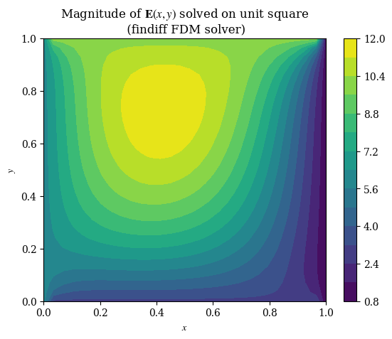
1abs_difference = np.abs(E - E_findiff)
1plt.imshow(correct_axes(abs_difference), interpolation="none", cmap="autumn")
2plt.title("Absolute difference between\n findiff and custom solvers")
3plt.colorbar()
4plt.show()
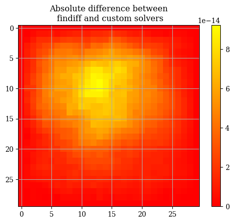
1abs_difference.max()
np.float64(9.237055564881302e-14)
The general differences between the findiff solver and the custom solver are very very miniscule on the order of \(\mathcal{E} \sim 10 \times e^{-13}\). Therefore we will use the two solutions interchangeably and consider them equivalent. If we inspect the solution, we can clearly see that the boundaries follow the boundary conditions:
1E[0, :] # E(0, y) = 6
array([6., 6., 6., 6., 6., 6., 6., 6., 6., 6., 6., 6., 6., 6., 6., 6., 6.,
       6., 6., 6., 6., 6., 6., 6., 6., 6., 6., 6., 6., 6.])
1E[-1,:] # E(1, y) = 1
array([1., 1., 1., 1., 1., 1., 1., 1., 1., 1., 1., 1., 1., 1., 1., 1., 1.,
       1., 1., 1., 1., 1., 1., 1., 1., 1., 1., 1., 1., 1.])
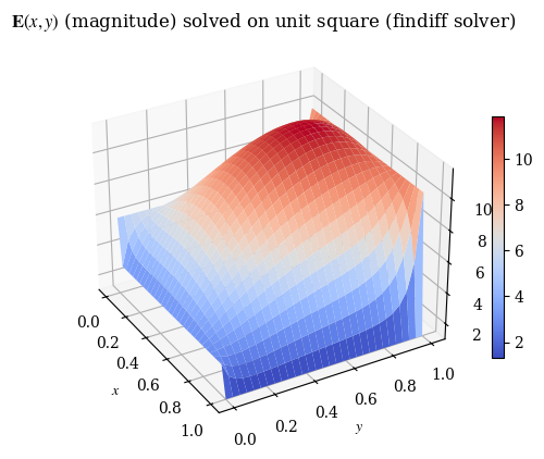
We can also verify with a 3D plot (where we now don’t need to do the transpose trick because we’re displaying 3D points and matplotlib is smart enough to figure that out):
1E_findiff.dtype
dtype('float64')
1# note this is V3
2plot_E(E_findiff, label=r"$\mathbf{E}(x, y)$ (magnitude) solved on unit square (findiff solver)", rot=-30)
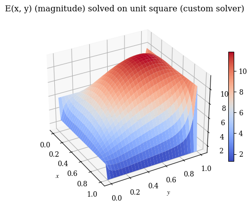
1# also V3
2plot_E(E, label="E(x, y) (magnitude) solved on unit square (custom solver)", rot=-30)
1# in function so as not to conflict with global vars
2def plotly_plot():
3    figdata = go.Surface(x=X, y=Y, z=E)
4    fig = go.Figure(figdata)
5    fig.update_layout(title="Numerical solution of Helmholtz equation")
6    fig.show()
1# uncomment to plot a live interactive solution
2# import plotly.graph_objects as go
3# plotly_plot()
The second test is the vector-valued version that uses the same coordinate transformations as the full version. However, do note that the Helmholtz equation’s vector components are independent of each other, meaning that the components can just as well be simulated separately (as two scalar PDEs) as together (as one vector PDE).
1def gen():
2    step = randint(0, squaren)
3    step2 = randint(0, squaren)
4    print(f"Generated test point ({step*dx:.3f}, {step2*dx:.3f}) corresponding to index [{step}, {step2}]")
5
6gen()
Generated test point (0.400, 0.600) corresponding to index [12, 18]
We test the validation points on the domain to compare against the FreeFEM version - note that this is because the finite element output is not on a regular mesh so cannot be compared value-by-value against the finite-difference result:
 1# convert real-space (x, y)
 2# coordinates to index (m, n)
 3# of the solution array
 4def convert_coord_index(x, y):
 5    x_idx = round(x*squaren)
 6    y_idx = round(y*squaren)
 7    # prevent out of bound
 8    # access errors
 9    if x_idx == squaren:
10        x_idx = -1
11    if y_idx == squaren:
12        y_idx = -1
13    return (x_idx, y_idx)
 1# unlike the freefem version, for this one
 2# we use the *index* locations of each point
 3# e.g. (1.0, 1.0) is equal to index [-1, -1]
 4# because it is the endpoint on both x and y
 5#
 6# for the ones where this method is a bit wonky, the
 7# convert_coord_index function is used
 8# which rounds the evaluation location to
 9# the closest set of [idx, idx] values
10cases = [
11    # boundary points
12    (0, 0.5),
13    (0.5, 0),
14    (1., 0.5),
15    (0.5, 1),
16    # center points
17    (0.25, 0.25),
18    (0.5, 0.5),
19    (0.75, 0.75),
20    # the three nonstandard points
21    # given by the gen() function above
22    (0.6, 0.),
23    (0.55, 0.562),
24    (0.663, 0.413)
25]
1testpoints = [convert_coord_index(*c) for c in cases]
 1def validate():
 2    results = [0 for i in range(len(testpoints))]
 3    for p_idx, p in enumerate(testpoints):
 4        i = p[0]
 5        j = p[1]
 6        # uncomment to show the corresponding index
 7        # print("Index:", f"({i}, {j})")
 8        if i == 0:
 9            x = 0
10        else:
11            x = i/squaren if i!= -1 else 1
12        if j == 0:
13            y = 0
14        else:
15            y = j/squaren if j!= -1 else 1
16        res = E[i][j]
17        print(f"On test point ({x:.3f}, {y:.3f}), result value {res}")
18        results[p_idx] = res
19    return results
1res = validate()
On test point (0.000, 0.500), result value 6.0
On test point (0.500, 0.000), result value 3.0
On test point (1.000, 0.500), result value 1.0
On test point (0.500, 1.000), result value 10.0
On test point (0.267, 0.267), result value 8.193004896091926
On test point (0.500, 0.500), result value 10.648553507303625
On test point (0.733, 0.733), result value 8.528249636148997
On test point (0.600, 0.000), result value 3.0
On test point (0.533, 0.567), result value 10.835052855936809
On test point (0.667, 0.400), result value 7.791280531797003
 1# from wave-parabolic-6-validation_4.edp
 2fem_results = [
 3    6.0,
 4    3.0,
 5    1.0,
 6    10.0,
 7    8.14275,
 8    11.3661,
 9    9.07413,
10    3.0,
11    11.4339,
12    8.78092
13]
1res_array = np.array(res)
2fem_res_array = np.array(fem_results)
1bar_x = np.arange(10)
1points_labels = [str(p) for p in testpoints]
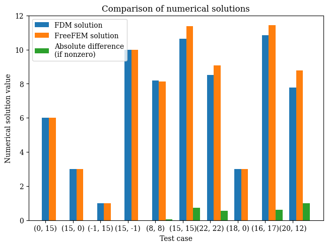
 1def plot_barchart(width=0.25, save=False):
 2    fig, ax = plt.subplots(layout='constrained')
 3    ax.set_title("Comparison of numerical solutions")
 4    ax.set_xlabel("Test case")
 5    ax.set_ylabel("Numerical solution value")
 6    p1 = ax.bar(bar_x, res_array, width=width, label="FDM solution")
 7    #ax.bar_label(p1, label_type="edge", fmt=lambda x: '{x:.2f}')
 8    p2 = ax.bar(bar_x + 0.25, fem_res_array, width=width, label="FreeFEM solution")
 9    #ax.bar_label(p2, label_type="edge", fmt=lambda x: '{x:.2f}')
10    p3 = ax.bar(bar_x + 0.5, np.abs(fem_res_array - res_array), width=width, label="Absolute difference\n(if nonzero)")
11    #ax.bar_label(p2, label_type="edge", fmt=lambda x: '{x:.2f}')
12    ax.set_xticks(bar_x, points_labels)
13    ax.legend()
14    plt.grid(False)
15    if save:
16        plt.savefig("validation-bar-chart.eps", dpi=600)
17    else:
18        plt.show()
1plot_barchart()
Vector-valued validation test#
We also want to do a simulation with the same boundary conditions but using a transformed coordinates system and vector-valued. As findiff can only solve scalar PDEs, in practice this means that we are solving 2 separate PDEs with different boundary conditions, and then combining them to get a vector-valued function. We are still using the same value of \(k\) and the same domain (of a unit square) as before. For the vector PDE, the coordinates in \((x, y)\) space are:
What we want is to convert to \((u, v)\) coordinates where \(u = e^x\) and \(v = e^y\). To preserve the same physical results, we must ensure that \(E(u, v) = E(x, y)\). which means re-expressing each of those boundary conditions in terms of functions \(E_u(u, v)\) and \(E_v(u, v)\). To do this we use the forward transforms \(E(u, v) = E(e^x, e^y)\). This means the function stays identical, and is simply expressed in different coordinates.
As an example, consider the first boundary condition \(E_x(x, 0) = 2\). The constant-valued outputs of the functions remains the same under the coordinate transformation, and the only thing that changes are the coordinates. That is to say, \(E_u(u, v) = E_x(u(x),v(y)\). For this, we substitute \(u(x)\) and \(v(y)\) into \(E_x(x, 0)\) as follows:
Doing so for each of the expressions, we obtain:
Where the domain \((x, y) \in [0, 1] \times [0, 1]\) becomes rescaled to \((u, v) \in [1, e] \times [1, e]\), as can be seen below:
1u_example = np.exp(x)
2print(u_example)
[1.         1.03508418 1.07139926 1.10898843 1.14789638 1.18816939
 1.22985534 1.27300381 1.3176661  1.36389534 1.41174649 1.46127646
 1.51254415 1.56561053 1.62053869 1.67739397 1.73624396 1.79715866
 1.8602105  1.92547447 1.99302816 2.06295193 2.13532891 2.21024517
 2.28778982 2.36805505 2.45113633 2.53713244 2.62614566 2.71828183]
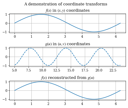
As a demonstration of the equivalence of solutions after a coordinate transform, consider the following change of variables \(x \to u = 3x + 5\) on a given function:
 1def test_coord_transform():
 2    # not from zero because we don't want 1/0
 3    x = np.linspace(0.01, 2*np.pi, 50)
 4    # u = u(x) the forwards transform
 5    u_of_x = lambda x: 3*x + 5 # u in terms of x
 6    # x = x(u) the backwards transform
 7    x_of_u = lambda u: (u - 5)/3 # x in terms of u
 8    fig = plt.figure()
 9    fig.suptitle("A demonstration of coordinate transforms")
10    ax1 = fig.add_subplot(3, 1, 1)
11    ax1.set_title("$f(x)$ in $(x, y)$ coordinates")
12    f = lambda x: np.sin(x)
13    # plot in x-space
14    ax1.plot(x, f(x))
15    # plot in u-space
16    ax2 = fig.add_subplot(3, 1, 2)
17    ax2.set_title("$g(u)$ in $(u, v)$ coordinates")
18    u = u_of_x(x)
19    g = lambda u: np.sin(u)
20    ax2.plot(u, g(u), linestyle="--")
21    ax3 = fig.add_subplot(3, 1, 3)
22    ax3.set_title("$f(x)$ reconstructed from $g(u)$")
23    ax3.plot(x, g(x_of_u(u)))
24    plt.subplots_adjust(hspace=0.75)
25    plt.show()
1test_coord_transform()
To solve the PDE in the new coordinates, the PDE itself must be converted to the new coordinates. By the chain rule, it can be shown that the new form the vector-valued PDE takes is given by:
Note that in the numerical programming we must expand out the partial derivatives. The expanded version of the Helmholtz operator is:
In addition, we will convert the boundary conditions respectively to:
1# forward transformations
2u_of_x = lambda x: np.exp(x)
3v_of_y = lambda y: np.exp(y)
1U = u_of_x(X)
2V = v_of_y(Y)
We can see that the domain \([0, 1] \times [0, 1]\) in \((x, y)\) maps to \([1, e] \times [1, e]\) in \((u, v)\) coordinates:
1U.min(), U.max()
(np.float64(1.0), np.float64(2.718281828459045))
Consider the first boundary condition \(E_x(x, 0) = 2\). We can show that it takes the form \(E_u(u, 1) = 2\) below:
1example_Ex_func = lambda x, y: 2
1example_Eu_func = example_Ex_func(u_of_x(x), v_of_y(y))
1example_Eu_func
2
 1# again incapsulate in function to prevent variable
 2# overwrite in global scope
 3# if refactoring is best to make a class for everything
 4def solve_transformed_helmholtz(x=x, y=y, k=k, shape=shape):
 5    u = u_of_x(x)
 6    v = v_of_y(y)
 7    du = u[1] - u[0]
 8    dv = v[1] - v[0]
 9    # not sure if we need to convert to meshgrid for this
10    U, V = np.meshgrid(u, v, indexing='ij')
11    d_du = FinDiff(0, du)
12    d_ddu = FinDiff(0, du, 2)
13    d_dv = FinDiff(1, dv)
14    d_ddv = FinDiff(1, dv, 2)
15    # helmholtz operator
16    # Helmholtz = Coef(U)*d_du + Coef(U**2)*d_ddu + Coef(V)*d_dv + Coef(V**2)*d_ddv + Coef(k**2)*Id()
17    Helmholtz = Coef(U)*(d_du + Coef(U)*d_ddu) + Coef(V)*(d_dv + Coef(V)*d_ddv) + Coef(k**2)*Id()
18    rhs = np.zeros(shape)
19    # we need separate boundary conditions for E_u and E_v components
20    # of the vector-valued PDE
21    bc_u = BoundaryConditions(shape)
22    bc_v = BoundaryConditions(shape)
23    # here note that we set based on the boundaries
24    # by index not by value
25    # the domain is [1, e] x [1, e]
26    bc_u[:, 0] = 2.0 # E_u(u, 1)
27    bc_u[:, -1] = 7.0 # E_u(u, e)
28    bc_u[0, :] = 0.5 # etc.
29    bc_u[-1, :] = np.pi
30
31    bc_v[:, 0] = 2*np.pi
32    bc_v[:, -1] = 3
33    bc_v[0, :] = 12
34    bc_v[-1, :] = 1
35
36    # PDE for u component of electric field
37    # the Helmholtz operator is identical for both PDEs
38    pde_u = PDE(Helmholtz, rhs, bc_u)
39    pde_v = PDE(Helmholtz, rhs, bc_v)
40    solution_u = pde_u.solve()
41    solution_v = pde_v.solve()
42    return solution_u, solution_v
1transform_u, transform_v = solve_transformed_helmholtz()
After solving for the components of \(\mathbf{E}\), we can visualize \(\mathbf{E}\) as a vector field as follows:
1def magnitude(E1, E2):
2    squared_norm = E1**2 + E2**2
3    return np.sqrt(squared_norm)
 1def plotE_uvspace(u=U, v=V, Usol=transform_u, Vsol=transform_v, desc=None, opacity=0.5):
 2    vec_density = 6 # plot one vector for every 10 points
 3    contour_levels = 12 # number of contours (filled isocurves) to plot
 4    transform_mag = magnitude(transform_u, transform_v)
 5    levels = np.linspace(transform_mag.min(), transform_mag.max(), contour_levels)
 6    # plot the filled isocurves
 7    plt.contourf(u, v, transform_mag, levels=levels)
 8    plt.colorbar()
 9    # plot the vectors
10    plt.quiver(u[::vec_density, ::vec_density], v[::vec_density, ::vec_density], Usol[::vec_density, ::vec_density], Vsol[::vec_density, ::vec_density], scale=400, headwidth=2, color=(1, 1, 1, opacity))
11    plt.xlabel("$u$")
12    plt.ylabel("$v$")
13    if not desc:
14        plt.title(r"$\mathbf{E}(u, v)$ solved on unit square in $(u, v)$ coordinates")
15    else:
16        plt.title(desc)
17    plt.show()
1plotE_uvspace()
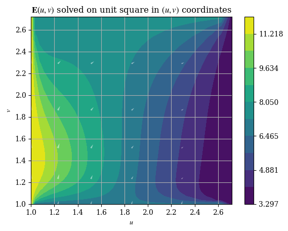
And the magnitude is respectively given by \(E = \|\mathbf{E}\| = \|E_u \hat{\mathbf{u}} + E_v \hat{\mathbf{v}}\| = \sqrt{E_u{}^2 + E_v{}^2}\), which can be plotted as shown:
1plt.imshow(correct_axes(magnitude(transform_u, transform_v)), interpolation="none")
2plt.title("Magnitude of $E(u, v)$ in $(u, v)$ coordinates")
3plt.colorbar()
4plt.show()
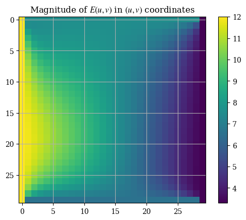
Note that the axes tickmarks can be ignored (they are not accurate) , as imshow() treats the input as if it were an image (which it obviously is not). We can validate the solution with the analytical expressions for the magnitude calculated from the boundary conditions for \(E_u\) and \(E_v\):
1E_prime_bottom = magnitude(2, 2*np.pi)
2E_prime_top = magnitude(7, 3)
3E_prime_left = magnitude(0.5, 12)
4E_prime_right = magnitude(np.pi, 1)
5print(f"Analytical values - top: {E_prime_top:.3f}, right: {E_prime_right:.3f}, bottom: {E_prime_bottom:.3f}, left: {E_prime_left:.3f}")
Analytical values - top: 7.616, right: 3.297, bottom: 6.594, left: 12.010
Which agree reasonably with the values shown in the plot. We will now do the comparison with the finite element solution for the validation.
 1# convert transformed-space (u, v)
 2# coordinates to index (m, n)
 3# of the solution array
 4def convert_coord_index_uv(u, v):
 5    u_idx = round((u-1)/(np.e-1)*squaren)
 6    v_idx = round((v-1)/(np.e-1)*squaren)
 7    # prevent out of bound
 8    # access errors
 9    if u_idx == squaren:
10        u_idx = -1
11    if v_idx == squaren:
12        v_idx = -1
13    return (u_idx, v_idx)
 1def validate_vector_uv():
 2    # here (u, v) is the domain [1, e] x [1, e]
 3    points = [
 4        [np.e/2, 1], # bottom
 5        [1, np.e/2], # left
 6        # the remainder are random points
 7        [1.3, 2.2],
 8        [1.7, 1.65],
 9        [2.4, 2.5]
10    ]
11
12    for p in points:
13        idx_u, idx_v = convert_coord_index_uv(*p)
14        transform_mag = magnitude(transform_u, transform_v)
15        res = transform_mag[idx_u, idx_v]
16        print(f"On test point ({p[0]:.3f}, {p[1]:.3f}), magnitude {res:.4f}")
1validate_vector_uv()
On test point (1.359, 1.000), magnitude 6.5938
On test point (1.000, 1.359), magnitude 12.0104
On test point (1.300, 2.200), magnitude 8.9589
On test point (1.700, 1.650), magnitude 8.6635
On test point (2.400, 2.500), magnitude 6.3954
To evaluate the solution \((x, y)\) coordinates, we remap each of the points from \((u, v)\) space to \((x, y)\) space, that is, applying the inverse transforms \(x(u) = \ln u\) and \(y(v) = \ln v\) (again the prime here denotes transformation, it is not a derivative symbol. As the solution is numerical (and therefore discrete), we must interpolate it to find \(\tilde{\mathbf{E}}(u, v)\) so that we can calculate the correct values according to the formula \(\mathbf{E}(x, y) = \tilde{\mathbf{E}}(x(u), y(v))\). For this we use scipy.optimize.curve_fit with a cubic polynomial in the form \(f(x, y) = ax^3 + by^3 + cx^2 y^2 + dx^2 + gy^2 + hxy + mx + nx + r\) on both components of \(\mathbf{E}'\):
1# have to flatten arrays to make this work
2def interpolation_func(X, a=1, b=1, c=1, d=1, g=1, h=1, m=1, n=1, r=1):
3    u_raw, v_raw = X
4    squaren = n # change based on the value of squaren globally
5    x = u_raw
6    y = v_raw
7    out = a*x**3 + b*y**3 + c*x**2*y**2 + d*x**2 + g*y**2 + h*x*y + m*x + n*x + r
8    return out.flatten()
1sol_u, cov_u = optimize.curve_fit(interpolation_func, (U.flatten(), V.flatten()), transform_u.flatten())
1sol_v, cov_v = optimize.curve_fit(interpolation_func, (U.flatten(), V.flatten()), transform_v.flatten())
We can then use the interpolated function as usual functions, E_u(u, v) and E_v(u, v) that can be given arguments, which represents \(\mathbf{E}'(u, v)\):
1# these take in vector-valued inputs i.e. you need to use np.meshgrid for them
2E_u = lambda u, v: interpolation_func((u.flatten(), v.flatten()), *sol_u).reshape(squaren, squaren)
3E_v = lambda u, v: interpolation_func((u.flatten(), v.flatten()), *sol_v).reshape(squaren, squaren)
4Emag_uv = lambda u, v: magnitude(E_u(u, v), E_v(u, v))
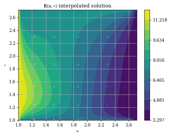
And we can plot it just like the original numerical solution:
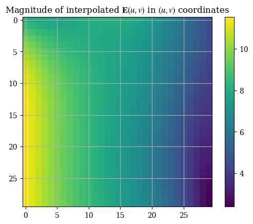
1plotE_uvspace(Usol=E_u(U, V), Vsol=E_v(U, V), desc=r"$\mathbf{E}(u, v)$ interpolated solution")
1plt.imshow(correct_axes(Emag_uv(U, V)), interpolation="none")
2plt.title("Magnitude of interpolated $\mathbf{E}(u, v)$ in $(u, v)$ coordinates")
3plt.colorbar()
4plt.show()
<>:2: SyntaxWarning: invalid escape sequence '\m'
<>:2: SyntaxWarning: invalid escape sequence '\m'
/tmp/ipykernel_2498/1675798493.py:2: SyntaxWarning: invalid escape sequence '\m'
  plt.title("Magnitude of interpolated $\mathbf{E}(u, v)$ in $(u, v)$ coordinates")
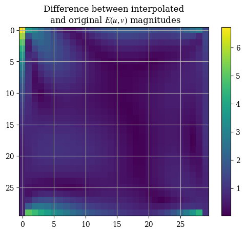
We can compare the interpolation functions’ accuracy with the original numerical solution:
1interpolation_err_u = np.abs(E_u(U, V) - transform_u)
2interpolation_err_v = np.abs(E_v(U, V) - transform_v)
For instance, we can find the general statistics of the maximum and mean error of the interpolation as compared to the numerical solution:
1interpolation_err_u.max()
np.float64(4.0804638937487)
1interpolation_err_v.max()
np.float64(5.348737680873402)
1interpolation_err_u.mean()
np.float64(0.3369530825804365)
1interpolation_err_v.mean()
np.float64(0.5749237657837586)
A histogram to be able to see how the error is spread out is best, but this will do for now. Here is a image plot of the same thing:
1interpolation_err = magnitude(interpolation_err_u, interpolation_err_v)
1cov_v.min()
np.float64(-6504718741215.889)
1plt.imshow(correct_axes(interpolation_err), interpolation="none")
2plt.title("Difference between interpolated\n and original $E(u, v)$ magnitudes")
3plt.colorbar()
4plt.show()
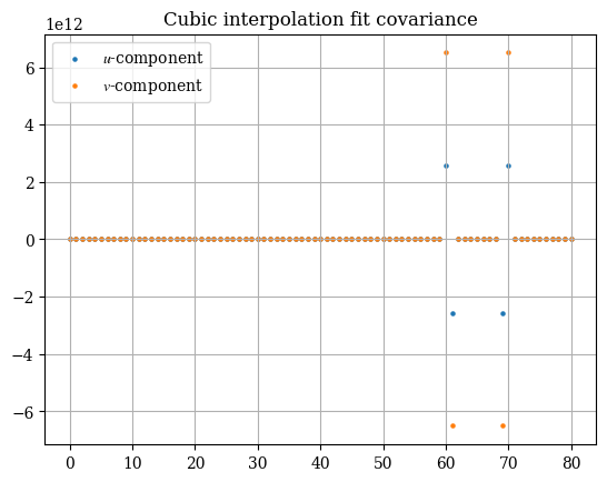
In addition, the output covariance is of interest to us. It is a measure of the spread of the interpolation scheme, and as such a low covariance is greatly desired. The covariance statistics are shown in the plot below. Curiously the fit seems to be almost perfect except for a few outlier points that are absolutely ridiculous:
1# todo: make the plot of the covariance work
2plt.title("Cubic interpolation fit covariance")
3plt.scatter(np.arange(np.prod(cov_u.shape)), cov_u.flatten(), label="$u$-component", s=5)
4plt.scatter(np.arange(np.prod(cov_v.shape)), cov_v.flatten(), label="$v$-component", s=5)
5plt.legend()
6plt.show()
For comparison we can evaluate the numerial vs interpolated solution next to each other on a common set of points:
1# we use pointwise variants of the interpolation function as opposed
2# to the one that takes vectorized input
3E_u_pointwise = lambda u, v: interpolation_func((u, v), *sol_u)
4E_v_pointwise = lambda u, v: interpolation_func((u, v), *sol_v)
5E_uv_pointwise = lambda u, v: float(np.sqrt(E_u_pointwise(u, v)**2 + E_v_pointwise(u, v)**2))
 1def validate_interpolate_vs_num_uv():
 2    # here (u, v) is the domain [1, e] x [1, e]
 3    points = [
 4        [(np.e-1)/2, 1], # bottom
 5        [1, (np.e-1)/2], # left
 6        # the remainder are random points
 7        [1.3, 2.2],
 8        [1.7, 1.65],
 9        [2.4, 2.5]
10    ]
11
12    print("Comparison of magnitudes (numerical vs interpolated)")
13    for p in points:
14        idx_u, idx_v = convert_coord_index_uv(*p)
15        transform_mag = magnitude(transform_u, transform_v)
16        res = transform_mag[idx_u, idx_v]
17        interp_res = E_uv_pointwise(*p)
18        print(f"On test point ({p[0]:.3f}, {p[1]:.3f}), numerical solution {res:.4f}, interpolated solution {float(interp_res):.4f}")
1validate_interpolate_vs_num_uv()
Comparison of magnitudes (numerical vs interpolated)
On test point (0.859, 1.000), numerical solution 6.5938, interpolated solution 13.3538
On test point (1.000, 0.859), numerical solution 12.0104, interpolated solution 11.5169
On test point (1.300, 2.200), numerical solution 8.9589, interpolated solution 8.5421
On test point (1.700, 1.650), numerical solution 8.6635, interpolated solution 7.4224
On test point (2.400, 2.500), numerical solution 6.3954, interpolated solution 5.6028
/tmp/ipykernel_2498/1914026686.py:5: DeprecationWarning: Conversion of an array with ndim > 0 to a scalar is deprecated, and will error in future. Ensure you extract a single element from your array before performing this operation. (Deprecated NumPy 1.25.)
  E_uv_pointwise = lambda u, v: float(np.sqrt(E_u_pointwise(u, v)**2 + E_v_pointwise(u, v)**2))
We can also check for the boundary conditions against their analytical values:
1print(f"Analytical values - top: {E_prime_top:.3f}, right: {E_prime_right:.3f}, bottom: {E_prime_bottom:.3f}, left: {E_prime_left:.3f}")
Analytical values - top: 7.616, right: 3.297, bottom: 6.594, left: 12.010
1half_u = (np.e - 1)/2
2half_v = (np.e - 1)/2
3E_interp_uv_top = E_uv_pointwise(half_u, np.e)
4E_interp_uv_right = E_uv_pointwise(np.e, half_v)
5E_interp_uv_bottom = E_uv_pointwise(half_u, 1)
6E_interp_uv_left = E_uv_pointwise(1, half_v)
/tmp/ipykernel_2498/1914026686.py:5: DeprecationWarning: Conversion of an array with ndim > 0 to a scalar is deprecated, and will error in future. Ensure you extract a single element from your array before performing this operation. (Deprecated NumPy 1.25.)
  E_uv_pointwise = lambda u, v: float(np.sqrt(E_u_pointwise(u, v)**2 + E_v_pointwise(u, v)**2))
1print(f"Interpolated values - top: {E_interp_uv_top:.3f}, right: {E_interp_uv_right:.3f}, bottom: {E_interp_uv_bottom:.3f}, left: {E_interp_uv_left:.3f}")
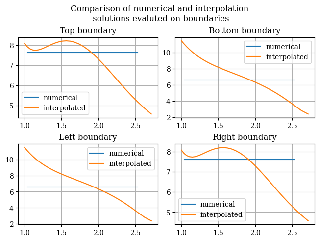
Interpolated values - top: 9.423, right: 2.298, bottom: 13.354, left: 11.517
It does seem that the interpolation is quite inadequate. To examine the issue further, we can plot the boundaries obtained from the original numerical solution as well as the transformation, which is shown below:
 1def compare_uv_bcs(Emag_numerical = magnitude(transform_u, transform_v), Emag_interp = Emag_uv(U, V), u=u_of_x(x), v=v_of_y(y), desc=None):
 2    fig = plt.figure(layout='constrained')
 3    if not desc:
 4        fig.suptitle("Comparison of numerical and interpolation\n solutions evaluted on boundaries")
 5    else:
 6        fig.suptitle(desc)
 7    spec = fig.add_gridspec(ncols=2, nrows=2)
 8    ax1 = fig.add_subplot(spec[0, 0])
 9    ax1.set_title("Top boundary")
10    # we use [1:-2] because we don't want the endpoints which are connected
11    # to the nodes of other boundaries
12    ax1.plot(u[1:-2], Emag_numerical[:, -1][1:-2], label="numerical")
13    ax1.plot(u, Emag_interp[:, -1], label="interpolated")
14    ax1.legend()
15    ax2 = fig.add_subplot(spec[0, 1])
16    ax2.set_title("Bottom boundary")
17    ax2.plot(u[1:-2], Emag_numerical[:, 0][1:-2], label="numerical")
18    ax2.plot(u, Emag_interp[:, 0], label="interpolated")
19    ax2.legend()
20    ax3 = fig.add_subplot(spec[1, 0])
21    ax3.set_title("Left boundary")
22    ax3.plot(v[1:-2], Emag_numerical[:, 0][1:-2], label="numerical")
23    ax3.plot(v, Emag_interp[:, 0], label="interpolated")
24    ax3.legend()
25    ax4 = fig.add_subplot(spec[1, 1])
26    ax4.set_title("Right boundary")
27    ax4.plot(v[1:-2], Emag_numerical[:, -1][1:-2], label="numerical")
28    ax4.plot(v, Emag_interp[:, -1], label="interpolated")
29    ax4.legend()
30    plt.show()
1compare_uv_bcs()
Due to this reason, an alternative approach will be used instead, that being a neural network. Due to the universal approximation theorem, neural networks are able to approximate any function. So we will use a neural network as a nonlinear approximator (interpolator) for the function.
To do this we combine the \(u\) and \(v\) vectors together into one vector \([(u_1, v_1), (u_2, v_2), (u_3, v_3), \dots (u_n, v_n)]\):
1trainX = np.stack((u_of_x(x), v_of_y(y))).T.reshape(-1, 2)
1trainX.shape
(30, 2)
We can validate this is correct by manually checking ordered pairs of \((u, v)\) coordinates:
1u_of_x(x)[0], v_of_y(y)[0]
(np.float64(1.0), np.float64(1.0))
1trainX[0]
array([1., 1.])
1u_of_x(x)[-1], v_of_y(y)[-1]
(np.float64(2.718281828459045), np.float64(2.718281828459045))
1trainX[-1]
array([2.71828183, 2.71828183])
Then we can preprocess the data with scikit-learn:
1scaler = StandardScaler()
1scaler.fit(trainX)
StandardScaler()In a Jupyter environment, please rerun this cell to show the HTML representation or trust the notebook.
On GitHub, the HTML representation is unable to render, please try loading this page with nbviewer.org.
StandardScaler()
1processed_trainX = scaler.transform(trainX)
1processed_trainX.shape
(30, 2)
We will also combine the \(E_u\) and \(E_v\) numerical solutions into one vector \([(E_{u_1}, E_{v_1}), (E_{u_2}, E_{v_2}), \dots, (E_{u_n}, E_{v_n})\). That means one \((u, v)\) coordinate maps to one value of \(\mathbf{E}'(u, v)\). For this we do have to be aware of what axis we are slicing through.
1np.stack((transform_u, transform_v)).shape
(2, 30, 30)
1# TODO FIX: make sure this is n elements
2trainY = np.stack((transform_u, transform_v)).reshape(2 * squaren, -1).T
1trainY.shape
(30, 60)
This is not as straightforward a process as it first seems due to the fact that scikit-learn only accepts 2D data for labels or for features at max. So what we will do is to reshape our \(2 \times n \times n\) array (because \(E_u\) and \(E_v\) each have \(n \times n\) elements) to \((2n, n)\), essentially slicing each \(n \times n\) array row-wise. The first n rows of the resulting array belowing to \(E_u\) and the next n rows belong to \(E_v\), and each of the rows has n elements. We then transpose, so the shape becomes \((2n, n) \to (n, 2n)\) to be able to get our labels to have the same shape across the first component as the features.
To turn the predicted results from the neural net back into a usable form, we transpose the prediction array \((n, 2n) \to (2n, n)\) and then split the 2n rows themselves into 2 sets of n rows. This means the final shape is \((2, n, n)\), i.e. two \(n \times n\) arrays, which we can then plot with imshow in matplotlib.
1processed_trainX.shape
(30, 2)
1trainY.shape
(30, 60)
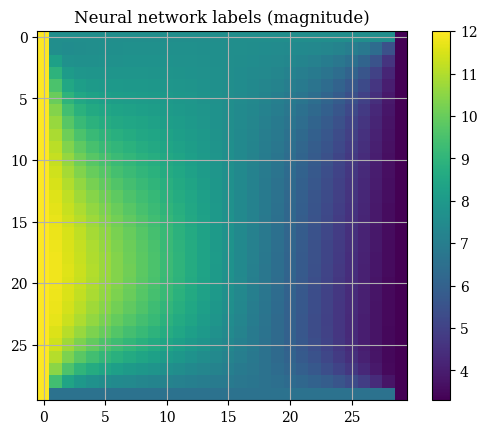
As a validation that our reshaping the array results in a valid result, we can run the prediction_to_grid() function directly on the data labels (i.e. the values of \(E_u\) and \(E_v\)) to show that it is correct.
1def prediction_to_grid(predictY):
2    # converts the output of the NN
3    # to two (n x n) grids for each
4    # of the two components of E
5    # (E_u and E_v)
6    # TODO this
7    E_u, E_v = predictY.T.reshape(2, squaren, -1)
8    return E_u, E_v
1# continue work here
2plt.title("Neural network labels (magnitude)")
3E_u_testgrid, E_v_testgrid = prediction_to_grid(trainY)
4plt.imshow(correct_axes(magnitude(E_u_testgrid, E_v_testgrid)), interpolation="none")
5plt.colorbar()
6plt.show()
1regr = MLPRegressor(random_state=1, activation="tanh", learning_rate="adaptive", max_iter=2500).fit(processed_trainX, trainY)
1regr
MLPRegressor(activation='tanh', learning_rate='adaptive', max_iter=2500,
             random_state=1)
In a Jupyter environment, please rerun this cell to show the HTML representation or trust the notebook. On GitHub, the HTML representation is unable to render, please try loading this page with nbviewer.org.
MLPRegressor(activation='tanh', learning_rate='adaptive', max_iter=2500,
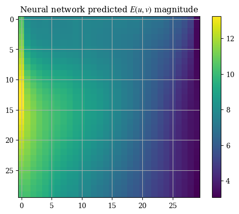
random_state=1)It may first seem that this approach works fine. We can see the boundary conditions being fixed on all of the four sides which is an important metric to determine the correctness of a solution. However, testing on the neural network-fit solution yields less-than-impressive results, with choppy and banded outputs that alternative between values and zeroes:
1E_predictions = regr.predict(processed_trainX)
2E_u_nn, E_v_nn = prediction_to_grid(E_predictions)
1plt.title("Neural network predicted $E(u, v)$ magnitude")
2plt.imshow(correct_axes(magnitude(E_u_nn, E_v_nn)), interpolation="none")
3plt.colorbar()
4plt.show()
And upon inspection we can immediately see why. If we take a look at our raw labels we see a bunch of discontinuities at the border where the two \(n \times n\) arrays meet:
1plt.title("Raw labels")
2plt.imshow(trainY)
3plt.show()
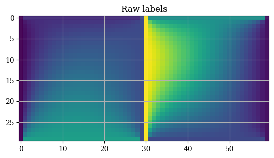
This is absolutely not what we want. So instead, just as with the interpolation method it might be a much better idea to train two separate neural networks, one for \(E_u\) and one for \(E_v\), so that the solutions are smooth and continuous which are much easier for neural networks to work with.
In addition, we want to directly map from a vector of \([(u_1, v_1), (u_2, v_2), (u_3, v_3), \dots (u_n, v_n)]\) of shape \((n, 2)\), to an output of shape \((n, n)\) for each of the neural networks. It may be the case that mapping from the meshgrid versions of \((u, v)\) leads to the banding behavior.
 1class NNInterpolation:
 2    def __init__(self, trainX=(u_of_x(x), v_of_y(y)), trainY=(transform_u, transform_v)):
 3        E_u, E_v = trainY
 4        u, v = trainX
 5        self.original_E_u = E_u
 6        self.original_E_v = E_v
 7        # we preprecess by running the train features through a
 8        # data scaler to rescale & regularize data for training
 9        # this should only be run once
10        # also no train/validation split because we're just
11        # using the NN as a model for the numerical solution
12        self.u_scaler = StandardScaler()
13        self.v_scaler = StandardScaler()
14        self.u_scaler.fit(u)
15        self.v_scaler.fit(v)
16        # preprocess the original data
17        self.U = self.u_scaler.transform(U)
18        self.V = self.v_scaler.transform(V)
19
20    def train(self, learning_rate="adaptive", max_iter=2500):
21        print("Training neural network...")
22        self.nn_u = MLPRegressor(random_state=1, learning_rate=learning_rate, max_iter=max_iter).fit(self.U, self.original_E_u)
23        self.nn_v = MLPRegressor(random_state=1, learning_rate=learning_rate, max_iter=max_iter).fit(self.V, self.original_E_v)
24
25    def check_shapes(self, U, V):
26        print("Checking dimensionality (must be 2D)...")
27        assert U.ndim == 2
28        assert V.ndim == 2
1nn_model = NNInterpolation()
2nn_model.train()
---------------------------------------------------------------------------
ValueError                                Traceback (most recent call last)
Cell In[103], line 1
----> 1 nn_model = NNInterpolation()
      2 nn_model.train()

Cell In[102], line 14, in NNInterpolation.__init__(self, trainX, trainY)
     12 self.u_scaler = StandardScaler()
     13 self.v_scaler = StandardScaler()
---> 14 self.u_scaler.fit(u)
     15 self.v_scaler.fit(v)
     16 # preprocess the original data

File /opt/hostedtoolcache/Python/3.12.5/x64/lib/python3.12/site-packages/sklearn/preprocessing/_data.py:878, in StandardScaler.fit(self, X, y, sample_weight)
    876 # Reset internal state before fitting
    877 self._reset()
--> 878 return self.partial_fit(X, y, sample_weight)

File /opt/hostedtoolcache/Python/3.12.5/x64/lib/python3.12/site-packages/sklearn/base.py:1473, in _fit_context.<locals>.decorator.<locals>.wrapper(estimator, *args, **kwargs)
   1466     estimator._validate_params()
   1468 with config_context(
   1469     skip_parameter_validation=(
   1470         prefer_skip_nested_validation or global_skip_validation
   1471     )
   1472 ):
-> 1473     return fit_method(estimator, *args, **kwargs)

File /opt/hostedtoolcache/Python/3.12.5/x64/lib/python3.12/site-packages/sklearn/preprocessing/_data.py:914, in StandardScaler.partial_fit(self, X, y, sample_weight)
    882 """Online computation of mean and std on X for later scaling.
    883
    884 All of X is processed as a single batch. This is intended for cases
   (...)    911     Fitted scaler.
    912 """
    913 first_call = not hasattr(self, "n_samples_seen_")
--> 914 X = self._validate_data(
    915     X,
    916     accept_sparse=("csr", "csc"),
    917     dtype=FLOAT_DTYPES,
    918     force_all_finite="allow-nan",
    919     reset=first_call,
    920 )
    921 n_features = X.shape[1]
    923 if sample_weight is not None:

File /opt/hostedtoolcache/Python/3.12.5/x64/lib/python3.12/site-packages/sklearn/base.py:633, in BaseEstimator._validate_data(self, X, y, reset, validate_separately, cast_to_ndarray, **check_params)
    631         out = X, y
    632 elif not no_val_X and no_val_y:
--> 633     out = check_array(X, input_name="X", **check_params)
    634 elif no_val_X and not no_val_y:
    635     out = _check_y(y, **check_params)

File /opt/hostedtoolcache/Python/3.12.5/x64/lib/python3.12/site-packages/sklearn/utils/validation.py:1050, in check_array(array, accept_sparse, accept_large_sparse, dtype, order, copy, force_writeable, force_all_finite, ensure_2d, allow_nd, ensure_min_samples, ensure_min_features, estimator, input_name)
   1043         else:
   1044             msg = (
   1045                 f"Expected 2D array, got 1D array instead:\narray={array}.\n"
   1046                 "Reshape your data either using array.reshape(-1, 1) if "
   1047                 "your data has a single feature or array.reshape(1, -1) "
   1048                 "if it contains a single sample."
   1049             )
-> 1050         raise ValueError(msg)
   1052 if dtype_numeric and hasattr(array.dtype, "kind") and array.dtype.kind in "USV":
   1053     raise ValueError(
   1054         "dtype='numeric' is not compatible with arrays of bytes/strings."
   1055         "Convert your data to numeric values explicitly instead."
   1056     )

ValueError: Expected 2D array, got 1D array instead:
array=[1.         1.03508418 1.07139926 1.10898843 1.14789638 1.18816939
 1.22985534 1.27300381 1.3176661  1.36389534 1.41174649 1.46127646
 1.51254415 1.56561053 1.62053869 1.67739397 1.73624396 1.79715866
 1.8602105  1.92547447 1.99302816 2.06295193 2.13532891 2.21024517
 2.28778982 2.36805505 2.45113633 2.53713244 2.62614566 2.71828183].
Reshape your data either using array.reshape(-1, 1) if your data has a single feature or array.reshape(1, -1) if it contains a single sample.
1E_u_nn, E_v_nn = nn_model.predict(U, V)
2tempvar = correct_axes(magnitude(E_u_nn, E_v_nn))
1plt.title("Neural network predicted $E(u, v)$ magnitude")
2plt.imshow(correct_axes(magnitude(E_u_nn, E_v_nn)))
3plt.colorbar()
4plt.show()
Note how we still see the banding, the outputs are not smooth and jump between two values. This means we need to do more testing to find a fitting method that respects the boundary conditions.
But this is not enough. We then need to apply the backwards transforms, which, like the forward transforms, preserves the features of the function, including having constant boundary conditions just like the original boundary conditions.
Finally, we evaluate the original function \(\mathbf{E}(x, y)\) through the interpolated version of \(\mathbf{E}'(u, v)\), via \(\mathbf{E}(x, y) = \mathbf{E}'(x(u), y(v))\). We have \(x(u) = \ln u, y(v) = \ln v\). Evaluating these on the arrays of \(u\) and \(v\) recovers \(\mathbf{E}(x, y)\).
1# backwards transforms
2x_of_u = lambda u: np.log(u)
3y_of_v = lambda v: np.log(v)
4
5E_x = E_u(x_of_u(U), y_of_v(V))
6E_y = E_v(x_of_u(U), y_of_v(V))
 1def plotE_xyspace(x=X, y=Y, E_x=E_x, E_y=E_y, desc=None, opacity=0.5):
 2    vec_density = 6 # plot one vector for every 10 points
 3    contour_levels = 12 # number of contours (filled isocurves) to plot
 4    E_mag = magnitude(E_x, E_y)
 5    levels = np.linspace(E_mag.min(), E_mag.max(), contour_levels)
 6    # plot the filled isocurves
 7    plt.contourf(x, y, E_mag, levels=levels)
 8    # plot the vectors
 9    plt.quiver(x[::vec_density, ::vec_density], y[::vec_density, ::vec_density], E_x[::vec_density, ::vec_density], E_y[::vec_density, ::vec_density], scale=400, headwidth=2, color=(1, 1, 1, opacity))
10    plt.xlabel("$x$")
11    plt.ylabel("$y$")
12    if not desc:
13        plt.title(r"$\mathbf{E}(u, v)$ transformed back to $(x, y)$ coordinates")
14    else:
15        plt.title(desc)
16    plt.colorbar()
17    plt.show()
1plotE_xyspace()
Compare these to the analytical boundary conditions:
 1def plotE_uvspace(u=U, v=V, Usol=transform_u, Vsol=transform_v, desc=None, opacity=0.5):
 2    vec_density = 6 # plot one vector for every 10 points
 3    contour_levels = 12 # number of contours (filled isocurves) to plot
 4    transform_mag = norm(transform_u, transform_v)
 5    levels = np.linspace(transform_mag.min(), transform_mag.max(), contour_levels)
 6    # plot the filled isocurves
 7    plt.contourf(u, v, transform_mag, levels=levels)
 8    # plot the vectors
 9    plt.quiver(u[::vec_density, ::vec_density], v[::vec_density, ::vec_density], Usol[::vec_density, ::vec_density], Vsol[::vec_density, ::vec_density], scale=400, headwidth=2, color=(1, 1, 1, opacity))
10    plt.xlabel("$u$")
11    plt.ylabel("$v$")
12    if not desc:
13        plt.title(r"$\mathbf{E}(u, v)$ solved on unit square in $(u, v)$ coordinates")
14    else:
15        plt.title(desc)
16    plt.colorbar()
17    plt.show()
1plotE_uvspace(u=X, v=Y, Usol=E_x, Vsol=E_y, desc="")
Which we may compare to our original boundary conditions, given by:
Finally, we can calculate the magnitude of the field via \(E(x, y) = \|\mathbf{E}(x, y)\|\). We can also validate this magnitude through the provided boundary conditions. For instance, \(E(x, 0) = \sqrt{E_x(x, 0)^2 + E_y(x, 0)^2} = \sqrt{4 + 4\pi^2} = 2\sqrt{1 + \pi^2}\). The full set of the boundary conditions of the magnitude field \(E\) are:
1bottom = norm([2, 2*np.pi])
2top = norm([7, 3])
3left = norm([0.5, 12])
4right = norm([np.pi, 1])
And the magnitude is plotted below:
1E_xy_mag = correct_axes(magnitude(E_x, E_y))
2plt.imshow(E_xy_mag)
3plt.colorbar()
4plt.show()