Antenna theory

At the beginning of our guide to our research, we went over the design of the ground-based power receivers, although our discussion was mostly conceptual. We will now introduce a theoretical analysis of the receiver stations, using the methods of antenna theory.

Antenna engineering

To be able to perform detailed theoretical analysis on the ground-based receiver stations, we must first understand the general ideas of antenna theory, as the receiver stations are arrays of large parabolic antennas. We recall that all electromagnetic waves are solutions of Maxwell’s equations. To solve for the electric and magnetic fields in the vecinity of an antenna, the full Maxwell equations - which can only be solved numerically in the vast majority of cases - are necessary for getting the most accurate results. However, there are some important analytical results and formulas we can derive before needing to reach for a computer, and these come from the field of electrical engineering.

Note

Before we start, a useful fact to keep in mind is that an antenna can generally be run both in receiving and transmitting mode (with a few modifications of its supporting circuitry/electronics, but not to the antenna itself). This means that a receiving antenna is just a transmitting antenna run in reverse. Thus, all results derived for receiving antennas also apply for transmitting antennas, and vice-versa.

To begin our study of antenna theory, let us introduce some terminology that is commonly-used in antenna theory. First, we introduce the solid angle. Think of a flashlight - note how its light spreads out in a cone. The spread of that cone can be measured in terms of solid angles, just like the spread between two lines (or vectors) can be measured in terms of regular angles. The unit of solid angle used in electrical engineering is the steradian, and just like radians, it is a dimensionless quantity. A full hemisphere is \(2\pi\) steradians, and a sphere (the steradian equivalent of 360 degrees but in 3D) is \(4\pi\) steradians. A visual example of the steradian is shown here:

We define the radiation intensity \(U\) of electromagnetic waves as the power carried in the wave passing through a given solid angle. We can calculate \(U\) from the magnitude of the Poynting vector \(S\) via:

\[ U = Sr^2 \]

Note that in general \(U\) depends on direction depends on direction, and using the the azimuthal and polar angles \(\theta\) and \(\phi\) (think longitude and latitude), we may write \(U(\theta, \phi) = S(\theta, \phi) r^2\). It has units of W/sr (watts per steradian).

Now we focus on more antenna-specific terminology. An antenna’s radiation pattern is a normalized function used to visually represent the intensity of the electromagnetic waves produced by an antenna in every direction. The radiation pattern function \(\operatorname{Rad}(\theta, \phi)\) is given by:

\[ \operatorname{Rad}(\theta, \phi) = \frac{U(\theta, \phi)}{U_\mathrm{max}} \]

Since the radiation pattern depends on the radiation intensity which depends on the Poynting vector’s magnitude, it requires finding an analytical (in rare cases) or numerical (most common) solution to Maxwell’s equations - more on numerical methods soon.

Another important quantity of antennas is their gain. When we first examined two analytical wave solutions of Maxwell’s equations, we looked at plane waves and more realistic waves that falloff \(\propto 1/r\) - the proper term for them is spherical waves. Far away from the source of the wave, spherical waves are a good approximation, and even plane waves are often sufficient. But no perfect spherical waves exist in the universe, because of Birkhoff’s theorem in electromagnetism. In addition, no antenna is perfectly efficient - all real antennas have some losses. So while real antennas can have approximately spherical wavefronts that move equally outward in all directions (we call the perfect case an isotropic radiator), spherical waves are an idealized approximation, a better one than plane waves, but still not physically possible.

Which brings us to the gain. The gain denoted \(G\), is the radiated power of an antenna relative to an ideal, lossless, isotropic radiator (which again, bears repeating, is not physically possible and is an idealization). In general, it is also a function of direction, that is, \(G = G(\theta, \phi)\). Given an antenna be fed with \(P_I\) watts of power (\(I\) for input power), its radiated power \(P_O\) over a certain area \(A = \displaystyle \int dA\) is given by:

\[ P_O = P_I G(\theta, \phi) \iint \frac{1}{4\pi r^2} dA \]

Mathematically, gain can be written as a ratio between the power radiated by an antenna and the power radiated by an ideal isotropic radiator (or analogously, the ratio between their respective radiation intensities). That is to say:

\[ G=\frac{P_O}{P_\mathrm{iso}} = \frac{U(\theta, \phi)}{U_\mathrm{iso}} = \frac{U(\theta, \phi)}{P_I / 4\pi} = 4\pi \frac{U(\theta, \phi)}{P_I} \]

Where in the previous equation we used the fact that an isotropic radiator has \(U = P_I / 4\pi\) as its radiation intensity, because remember, radiation intensity is power per unit solid angle, not power per unit area. All of these compound definitions means that we can write the gain in terms of the magnitude of the Poynting vector \(S\) via:

\[ G(\theta, \phi) = 4\pi \frac{Sr^2}{P_I} \]

And thus we can write the radiated power \(P_O\) as:

\[ P_O = 4\pi Sr^2 \iint \frac{1}{4\pi r^2} dA = Sr^2 \iint \frac{1}{r^2} dA \]

Luckily, there is an analytical expression for the maximum gain of a parabolic antenna (remember this is the same whether the antenna is run as a receive or transmitter), and parabolic antennas are the main type the microwave-based power transfer approach uses. While parabolic antennas have complicated gain functions, the maximum of their gain function is given by a simple expression:

\[ G_\mathrm{max} = \left(\frac{2\pi R}{\lambda}\right)^2 e_A \]

Where \(e_A\) is a constant known as the effective aperture, typically marked on the antenna by the manufacturer, but reasonably well-approximated by a value between 0.5-0.7 (this is the typical range of aperture efficiencies), and can be found by doing controlled tests with the antenna. Also: note that the gain is often given in decibels, which are a dimensionless unit expression for logarithmic scales, where \(G_\mathrm{dB} = 10 \log_{10}G\). This is because raw gain measurements can quickly explode into the millions for large parabolic antennas and so to keep numbers within a reasonable range, it is better to work with decibels than the pure numerical value of the gain.

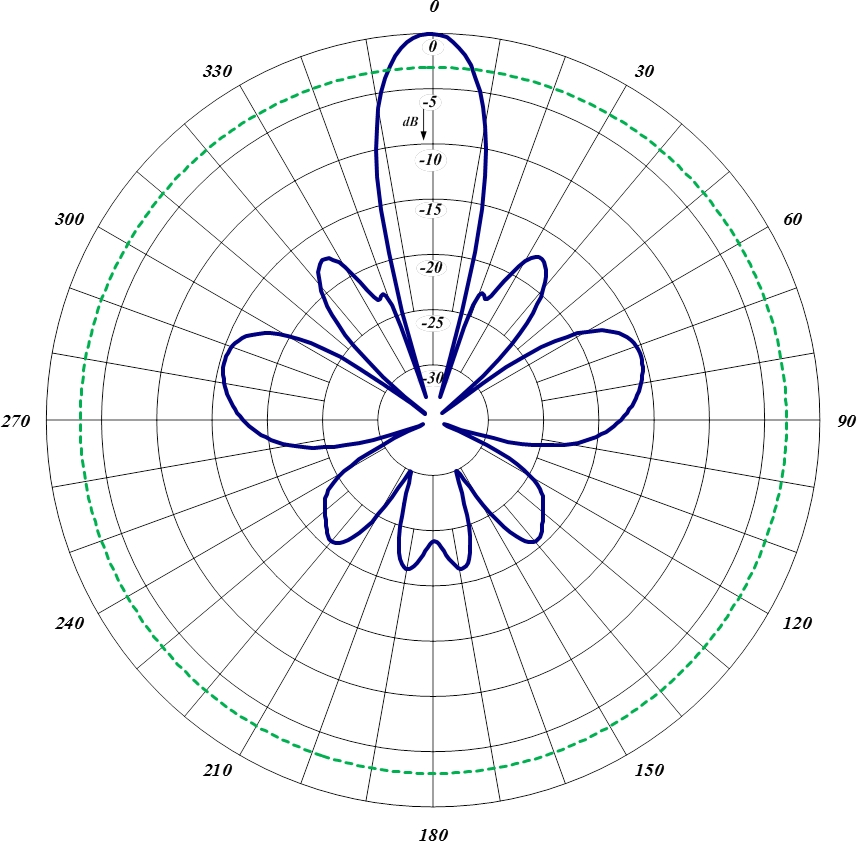
For a parabolic antenna, there exists an analytical solution for the radiation pattern (one may read more on this solution on Wikipedia), and it is given by:

\[ \operatorname{Rad}(\theta) = \frac{2 \lambda}{\pi D} \frac{J_1(2\pi R/\lambda)\sin \theta}{\sin \theta} \]

Where \(J_1(\theta)\) is a Bessel function of the first kind, defined by:

\[ J_1(\theta) = \frac{1}{\pi} \int_0^\pi \cos(n\tau - \theta \sin \tau)~d\tau \]

Here’s a plot of the radiation pattern, courtesy of Comprod, a seller of antennas and other digital equipment, notice they use decibels otherwise the gain would be extreme and be almost entirely directed towards the direction the parabolic antenna is facing:

The crucial parameter to successful power transfer is to maximize the gain in the direction of reception for the ground-based receiver station antennas. This involves two things:

1. Reducing losses in general to increase efficiency, as greater inefficiencies means lower gain

2. Doing multiple iterations of the antenna design, computing the radiation pattern each time, and trying to tighten the radiation pattern around the transmission direction until it is highly focused without the “lobes” that protrude outwards and represent lost power.

Antenna simulations

With an overview of antenna theory, we have gained a basic understanding that we can apply to analyze our power receiver stations. But all theoretical models are idealizations, and while they serve as good sanity-checks and provide analytical results, these often require heavy use of approximations or only apply in idealized scenarios. Further, some problems are completely unsolvable by using purely analytical means. This is why utilizing numerical methods to perform computer-based simulations are such a big part of our work at Project Elara.

We will go into the general theory of numerical methods for PDEs later, but we will begin with a direct application of a numerical method for designing and simulating antennas: using finite element analysis to solve the electromagnetic wave equation and Helmholtz equation.

Finite element analysis

Finite element analysis (also called the finite element method) is the general name for a wide class of approaches that solve partial differential equations by approximating the solution with piecewise functions. The goal of finite element analysis is to find the correct coefficients for the piecewise function(s) that satisfies an integral form of the PDE. This particular integral form is called a weak form (or variational form), and relies on using methods from vector calculus to rewrite a PDE in a specific form that is easy to integrate by computer. Discretizing the integrals results in a system of linear equations, which can be solved using the methods of numerical linear algebra.

Warning

This subsection is very mathematically-heavy, so feel free to skip this section if you don’t plan to work on simulations or other applications relying on numerical methods.

As a reminder, our PDEs to be solved for are two wave equations for the electric and magnetic fields:

\[\begin{split} \frac{\partial^2}{\partial t^2} \begin{pmatrix} \mathbf{E} \\ \mathbf{B} \end{pmatrix} = c^2 \nabla^2 \begin{pmatrix} \mathbf{E} \\ \mathbf{B} \end{pmatrix} \end{split}\]

As well as the Helmholtz equation for the electric and magnetic fields (note that these are for the time-independent components of each field, unlike the wave equation, which is time-dependent):

\[\begin{split} \begin{align*} \nabla^2 \mathbf{E}(\mathbf{r}) + k^2 \mathbf{E}(\mathbf{r}) = 0 \\ \nabla^2 \mathbf{B}(\mathbf{r}) + k^2 \mathbf{B}(\mathbf{r}) = 0 \end{align*} \end{split}\]

To perform finite element analysis, we must perform three general steps:

1. Rewrite the PDE + boundary conditions (which is called the strong form) into an equivalent integral equation (which is called the weak form)

2. Simplify the weak form as much as we can with vector calculus identities

3. Input the weak form into a finite element software of choice, plus the boundary conditions, then let the software solve for us

To get the weak form from the wave equation, we multiply both sides of each PDE by a test function \(\Phi\) which is vector valued, then integrate over the 3D spatial domain \(\Omega\) that includes everywhere within the boundaries. Note that we did not include time in the domain even though there are time derivatives - to do so would be computationally expensive. Rather, we can take out the time derivatives, and leave them there for now, we will replace the time derivatives with a numerical approximation later. We also have the helpful fact that the two PDEs are identical in form, so we will just work with the electric field wave equation, because the results for the magnetic field wave equation are identical other than replacing \(\mathbf{E}\) with \(\mathbf{B}\). Let’s restate the wave equation for electric fields:

\[ \displaystyle \frac{\partial^2 \mathbf{E}}{\partial t^2} = c^2 \nabla^2 \mathbf{E} \]

Remember that this is written in vector calculus notation and expands to:

\[ \frac{\partial^2 \mathbf{E}}{\partial t^2} = c^2 \left(\frac{\partial^2 \mathbf{E}}{\partial x^2} + \frac{\partial^2 \mathbf{E}}{\partial y^2} + \frac{\partial^2 \mathbf{E}}{\partial z^2}\right) \]

Which is itself shorthand for a system of three PDEs:

\[\begin{split} \begin{align}\frac{\partial ^2E_x}{\partial t^2} &= c^2 \left(\frac{\partial ^2E_x}{\partial x^2} + \frac{\partial ^2E_x}{\partial y^2} + \frac{\partial ^2E_x}{\partial z^2}\right) \\ \frac{\partial ^2E_y}{\partial t^2} &= c^2 \left(\frac{\partial ^2E_y}{\partial x^2} + \frac{\partial ^2E_y}{\partial y^2} + \frac{\partial ^2E_y}{\partial z^2}\right) \\ \frac{\partial ^2E_z}{\partial t^2} &= c^2 \left(\frac{\partial ^2E_z}{\partial x^2} + \frac{\partial ^2E_z}{\partial y^2} + \frac{\partial ^2E_z}{\partial z^2}\right) \\ \end{align} \end{split}\]

When we’re doing mathematical manipulations, it helps to not get too lost in notation and lose track of the underlying things we’re operating on. In addition, when working with vector-valued PDEs or PDE systems, it is much-preferred to use tensors. Here, the Einstein summation convention is implied, and everything is assumed to be in a Euclidean space (so upper and lower indices are related by \(A^j = A_i \delta^{ij}\) where \(\delta^{ij} = \delta_{ij}\) is the Kronecker delta. Writing the electric field wave equation in tensor form, we have:

\[ \partial^2_t E^i = c^2 \partial^j \partial_j E^i \]

Where \(\partial^2_t = \displaystyle \frac{\partial^2}{\partial t^2}\). Again, we will treat time derivatives separately via difference quotient approximations so we will just leave them there and not try to simplify the left-hand side. After all, the time dimension is a very regular one-dimensional domain and easy to use just a finite difference with, unlike the highly irregular spatial domain. We multiply (vector multiplication is dot product here) by vector test function \(\Phi_i\) to everything, so we get:

\[ \Phi_i \partial^2_t E^i = c^2 \Phi_i\partial^j \partial_j E^i \]

And then we integrate everything to get:

\[ \int_\Omega \Phi_i \partial^2_t E^i~dV = c^2 \int_\Omega \Phi_i\partial^j \partial_j E^i dV \]

Theoretically speaking, this is fine for an integral equation. But for solving, we would rather want a lower-order - ideally, first order - expression, and reduce the dimensionality of the integrals which improves computational performance. You could look up a table of vector calculus identities. Or, you can do it purely with tensors, by using integration by parts. Recall that the product rule is given by:

\[ \frac{\partial}{\partial x^a} (uv) = v \frac{\partial u}{\partial x^a} + u \frac{\partial v}{\partial x^a} \]

Be careful to note that all terms of the product rule must use the same index. You cannot have a \(\partial_a\) in one term and \(\partial_b\) in another term. Writing in compact tensor notation, we can rewrite as \(\partial_a (uv) = v\,\partial_a u + u\,\partial_a v\), which we can rearrange to \(u\, \partial_a v = \partial_a (uv) - v\, \partial_a u\). The expression we want to simplify is \(\Phi_i\partial^j \partial_j E^i\), which is in the form \(u \, \partial_a v\) where \(u = \Phi_i\) and \(\partial_a v = \partial^j \partial_j E^i\). So \(v = \partial_j E^i\) and \(\partial_a u = \partial^j \Phi_i\), and thus:

\[ \Phi_i\partial^j \partial_j E^i = \partial^j (\Phi_i \partial_j E^i) - (\partial_j E^i)(\partial^j \Phi_i) \]

We can drop the brackets on the second term, so long as we remember that it is a product:

\[ \Phi_i\partial^j \partial_j E^i = \partial^j (\Phi_i \partial_j E^i) - \partial_j E^i \partial^j \Phi_i \]

Now, substituting this back into the right-hand side term, we obtain:

\[ \int_\Omega \Phi_i \partial^2_t E^i~dV = c^2 \int_\Omega \Phi_i\partial^j \partial_j E^i dV = c^2 \int_\Omega \partial^j (\Phi_i \partial_j E^i) - \partial_j E^i \partial^j \Phi_i\,dV \]

Using the Kronecker delta on the right-hand side term, we can rewrite \(E^i = \delta^i {}_j E^j\). So:

\[ \int_\Omega \Phi_i \partial^2_t E^i~dV = c^2 \int_\Omega \partial^j (\Phi_i \partial_j E^i) - \partial_j E^i \partial^j \Phi_i\,dV \]

We can split the right-hand side integral into two for convenience:

\[ \int_\Omega \Phi_i \partial^2_t E^i~dV = c^2 \int_\Omega \partial^j (\Phi_i \partial_j E^i)\,dV - c^2\int \partial_j E^i \partial^j \Phi_i\,dV \]

Notice the term \(\partial^j (\Phi_i \partial_j E^i)\). We can write it as \(\partial^j B_j\) where \(B_j = \Phi_i \partial_j E^i\). But by the Divergence Theorem:

\[ \int_\Omega \partial^j B_j\,dV = \int_{\partial \Omega} B_j dA^j \]

This may look more familiar when written in standard vector calculus notation:

\[ \int_\Omega \nabla \cdot \mathbf{B}~dV = \int_{\partial \Omega} \mathbf{B}\cdot d\mathbf{A} \]

This is great because we can reduce the dimensionality of the integral from a volume integral to a surface integral! Therefore we arrive at:

\[ \int_\Omega \Phi_i \partial^2_t E^i \, dV = c^2 \int_{\partial \Omega} \Phi_i \partial_j E^i \,dA^j - c^2\int_\Omega \partial_j E^i \partial^j \Phi_i\,dV \]

Which we can write in more typical notation as:

\[ \int_\Omega \Phi \cdot \frac{\partial^2 \mathbf{E}}{\partial t^2}~dV = c^2 \left[ \int_{\partial \Omega} \Phi \cdot \nabla_J \mathbf{E}~d\mathbf{A} - \int_\Omega \nabla_J \mathbf{E} : \nabla_J \Phi~dV \right] \]

Where : is the double dot product (tensor product for matrices). If we move all the terms to one side, we have:

\[ \int_\Omega \Phi \cdot \frac{\partial^2 \mathbf{E}}{\partial t^2}~dV - c^2 \int_{\partial \Omega} \Phi \cdot \nabla_J \mathbf{E}~d\mathbf{A} + c^2 \int_\Omega \nabla_J \mathbf{E} : \nabla_J \Phi~dV = 0 \]

Notice that we have a time derivative on the left. As we integrate only over space, we must timestep our weak form, meaning we have to discretize the derivative and compute the weak form for every discrete \(t\). Using a table of derivative approximations, such as on this website, we may choose the following approximation for the second derivative:

\[ \frac{\partial^2 \mathbf{E}}{\partial t^2} = \frac{\mathbf{E}(t_{n+1}, \mathbf{x}) - 2\mathbf{E}(t_n, \mathbf{x}) + \mathbf{E}(t_{n - 1}, \mathbf{x})}{\Delta t^2} \]

We have to be careful because the \(\mathbf{E}(t, \mathbf{x})\) that appears in the variational form is actually the unknown next time-step \(\mathbf{E}^{n + 1}\) that we want to calculate. So in order to make this explicit, the variational form is given by:

\[ \int_\Omega \Phi \cdot \frac{\mathbf{E}^{n+1} - 2\mathbf{E}^{n} + \mathbf{E}^{n-1}}{\Delta t^2}~dV - c^2 \int_{\partial \Omega} \Phi \cdot \nabla_J \mathbf{E}^{n+1}~d\mathbf{A} + c^2\int_\Omega \nabla_J \mathbf{E}^{n+1} : \nabla_J \Phi~dV = 0 \]

This is the most general simplified weak form of the wave equation. Beyond this point, we need to individually-substitute each of the boundary conditions into the variational form, which is dependent on the specific electromagnetics problem, and the rest is software-specific. For inputting these weak forms into software, it is important to know the four categorizations of weak-form terms:

• Bilinear terms are terms that involve the function to be solved for

• Linear terms are terms that don’t involve the function to be solved for

• Domain terms are terms integrated over \(\Omega\) (the entire domain)

• Boundary terms are terms integrated over \(\partial \Omega\) (the boundary of the domain)

We must take special care when identifying the terms in the wave equation, because the terms are not as simple as they seem. As \(\mathbf{E}^{n + 1}\) is the function we’re computing on every time-step based on the calculated result \(\mathbf{E}^n\) from the previous time-step, all terms that involve \(\mathbf{E}^{n + 1}\) are bilinear (as we are solving for that), while all the terms that contain \(\mathbf{E}^n\) and \(\mathbf{E}^{n - 1}\) are linear (as we are not solving for them). (Yes, this is quite confusing).

We should also note that by applying the same process to the Helmholtz equation \(\nabla^2 \mathbf{E} + k^2 \mathbf{E} = 0\) we can also find its weak form, which we will not derive to avoid making this page overly long. The result is:

\[ - \int_\Omega \nabla_J \mathbf{E} : \nabla_J \Phi\, dV + k^2 \int_\Omega \Phi \cdot \mathbf{E}\,dV + \int_{\partial \Omega} \Phi \cdot \nabla_J \mathbf{E} \,d\mathbf{A} = 0 \]

After substituting the boundary conditions into the problem and setting the domain, the weak form of the PDE can be substituted into a variety of software packages designed to find numerical solutions by the finite element method. We use two major ones in Project Elara: FreeFEM, which is a standalone software, and FEniCS, which is a Python library. Both software packages are open-source, feature-rich, and used extensively by scientists and engineers.