Lasers and laser physics#
As we’ve covered previously, a key component in our proposed space swarm system is the maser (microwave laser) that transmits the captured energy of sunlight back to Earth. Designing a laser to meet the high demands of our use case is an immense engineering challenge, which we hope to accomplish with research breakthroughs and technological innovation. But before examining the specifics of state-of-the-art laser technology, let us first go over the essential quantum theory behind how lasers work.
Operating principles of lasers#
We know from the quantum model of the hydrogen atom that electrons can have different states. As each state is an eigenstate of the Hamiltonian, the (non-degenerate) states also have different energies. If an atom absorbs a photon, for instance, the atom can jump from its ground state, which we write as \(|1\rangle\), to a higher-energy excited state \(|2\rangle\). Meanwhile, an atom can also decay to its ground state by emitting a photon, with the difference in the energies \(E_2 - E_1\) between the excited state and the ground state being the energy of this photon. While atoms, in general, have a multitude of states (and more than one excited state), this two-state approximation is good enough for a lot of theoretical analysis. A diagram of the two-state atomic system is shown below:

Precisely when the decay happens is random, and it may occur spontaneously (i.e. without anything external causing it), so we call it spontaneous emission. We do know, however, that this process follows a probabilistic law, first derived by Einstein in 1916. Let us assume we are studying a certain group of electrons. Let \(N_2(t)\) be the expected number of electrons in a higher energy state \(|2\rangle\). Over time, these electrons will spontaneously decay to a lower energy state \(|1\rangle\), such that \(N_2(t)\) follows the differential equation:
Where \(A_{21}\) is called the Einstein A coefficient, and is approximately the probability that an electron will decay from \(|2\rangle \to |1\rangle\) per unit time. Remember, this is probabilistic, as in \(N_2(t)\) is the expected number of electrons in the excited state, as in, it is most likely that at time \(t\) there are \(N_2\) electrons that are in the excited state \(|2\rangle\). This differential equation is just an exponential decay whose solution is:
Remember that spontaneous emission is fundamentally random in nature; they follow general probabilistic rules but those are simply probabilities. But we don’t want that, we want emission of photons that we can control.
For this, we need stimulated emission. First, we bring the atom to its excited state by surrounding it with an externally-applied energy source. When this energy source is another electromagnetic field (e.g. flash lamp, arc lamp, sunlight, even an LED) is called optical pumping. It is in fact possible to use one laser to optically pump another laser - in fact, this is often the most efficient method of pumping a laser, and can be used to take a laser beam of one wavelength to be able to produce a laser beam of another wavelength.
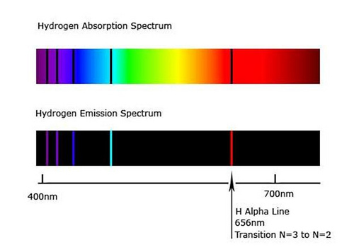
The wavelength used in optical pumping does not necessarily have to be the same wavelength that is emitted. The chief requirement is that the optical source used in optical pumping matches one of the absorption lines of the atom (or molecule, or molecular gas lasers). For instance, hydrogen absorbs (and correspondingly, also emits) wavelengths of 656 nm (red), 486 nm (cyan), 434 nm (blue), 410 nm (violet), and a variety of other wavelengths in the UV band, among others, as shown below:
But while these absorption lines at the most well-known, they are not its only absorption lines, because, due to fine structure and hyperfine structure (the splitting of energy levels due to complex quantum effects), other types of transitions are possible, including the 21 cm absorption line (and emission line) in the microwave spectrum.
When an atom has been raised to its excited state by some energy source, a passing photon that has energy \(\Delta E = E_2 - E_1\) will stimulate the decay of the atom from its excited-state \(|2\rangle\) to its ground-state \(|1\rangle\), releasing another further photon of energy \(\Delta E\) with the exact same properties as the passing photon. The passing photon that stimulated the transition between the states, however, is not absorbed, meaning that now there are two photons of energy \(\Delta E\). These two photons can then pass by one atom each, triggering the release of two more photons from each atom, so four photoms after. The process continues, with emitted photons stimulating another atomic transition which would emit another photon, repeating the process over and over to create a cascade of electromagnetic radiation. Thus, we have the laser: an acronym for light amplification by simulated emission of radiation.
Crucially, stimulated emission needs a large population (number of atoms) to be already in the excited state - otherwise, we would see mostly spontanenous emission rather than stimulated emission. Pumping - that is, introducing an external energy source - is what allows stimulated emission to dominate over spontaneous emission, as the population of the excited state is greater than the population of the ground state, which we call a population inversion. We may quantify the expected number of atoms \(N_2\) in the higher energy state \(|2\rangle\) with the following differential equation:
Where \(\nu\) is the frequency of the radiation, \(\rho(\nu)\) is Planck’s law at temperature \(T\), and \(B_{21}\) is called the Einstein B coefficient (which we’ll derive later), which again is a probabilistic measure of decay from \(|2\rangle \to |1\rangle\):
An annotated sketch showing the interrelationships between each of these mathematical relations is shown below:

As an example of how this works in practice, the He-Ne laser, a common type of laser operating in the visible spectrum, uses a mixture of helium and neon gas within an optical chamber. An electrical discharge is created in the chamber between the cathode (positive end) and anode (negative end), which acts as an energy source (laser pump source), causing the gas to become a plasma where the electrons are free to move around. The electrons randomly collide with the helium atoms, transferring energy and bringing the helium to an excited state. The helium atoms also collide with the neon atoms, bringing the neon atoms to an excited state and allowing the helium atoms to decay to a lower-energy state. These atoms in excited states provide the conditions for stimulated emission to occur: when one atom decays to lower-energy states and release a photon, another atom would release another photon by stimulated emission. A reflective mirror at one end of the chamber and a semi-transparent mirror at the end reflects the light back and forth, repeating this process over and over and amplifying the light by re-concentrating energy into the gain medium, ensuring that atoms are raised to the excited state, and continuing the cyle of stimulated emission. At a certain point, this cycle of continuous amplification through stimulated emission has progressed far enough that photons escape the optical cavity and begin to pass through the semi-transparent mirror, which is the laser beam we see.
In a laser, light is fundamentally quantized - that is the prerequisite that allows stimulated emission in the first place. Given that photons are quanta of the electromagnetic field, the full picture of laser dynamics would in theory require a quantum treatment of electromagnetism, that is, quantum electrodynamics. However, the actual quantum-mechanical workings of lasers can be approximately treated as separate from the electromagnetic field produced within it. This means that we can actually describe use classical electromagnetic theory - and specifically the Gaussian beam solution to the Helmholtz equation - and use it to derive quantum results. And indeed, this is what we will do.
Theoretical analysis#
Lasers are devices that rely on stimulated emission to emit light - in fact, LASER is an acronym for “light amplification by stimulated emission of radiation”. This is in contrast with lightbulbs, stars, or blackbody radiators, which which operate by either stimulated emission or absorption. A laser relies on creating the optimal conditions for spontaneous emission to occur.
Quantum mechanically-speaking, a laser can be classified as a multi-state system that undergoes transitions between its states. This requires more advanced methods compared to time-independent systems, which do not have transitions between states, and therefore have constant probabilities to be in each of their possible states . To analyze lasers, we must use time-dependent perturbation theory, where the probabilities of each state are dependent on time.
In our case, let us first discuss the generalized theoretical approach to analyzing lasers; we will then discuss one of the simplest analytical solutions that corresponds to a real-world laser system: the ammonia maser.
Consider a two-state laser whose gain medium is pumped by an electromagnetic field. Such a system can occupy two states: the ground state, which (out of convenience) we will call \(|1\rangle\), and the excited state, which we will call \(|2\rangle\). The general state of the system, assuming that transitions are forbidden, is given by:
where \(|1\rangle, |2\rangle\) are eigenstates of the system’s Hamiltonian assuming no transitions (which we will call \(\hat H_0\)):
Now, this is only the case if transitions are forbidden - but we know that transitions between the ground state and excited states do certainly exist. Therefore, we must add time-dependence to the system, which means \(c_1, c_2\) must become functions of time \(c_1(t), c_2(t)\):
Further, since a laser is pumped by an electromagnetic field, we must adjust our Hamiltonian. Our previous Hamiltonian \(\hat H_0\), which was time-independent, must be adjusted to accomodate an extra term \(\hat H_1\) which describes the time-oscillating electromagnetic field. Therefore: