Classical mechanics, Part 1

“The important thing is to never stop questioning.”

Albert Einstein

For over 200 years, before the advent of 20th century relativistic and quantum physics, our view of the world was dominated by classical mechanics. From the foundation laid by Newton to the work of Lagrange and Euler and the masterminds of Faraday and Maxwell, classical mechanics set out to describe the world around us through concrete, physical laws, and still does so brilliantly. This guide aims to explain classical mechanics in as simple and elegant a way as possible, hopefully allowing you to soon have a working knowledge of mechanics with which to do physics.

Kinematics

We can describe the location of a point through what is known as a position function. The position function \(s(t)\) describes the location of an object through space at any given time. For example, imagine a position function as follows:

\[ s(t) = 3t^{3}-5t+1 \]

We adopt the convention in physics that positive numbers are used for positions to the top or right, and negative numbers are used for positions to the left or bottom.

At \(t = 0\), \(s(t) = 1\), which means that the object is 1 meter to the right of the origin at that time. At \(t = 1\), \(s(t) = -1\), which means the object is 1 meter to the left of the origin. At \(t = 2\), \(s(t) = 15\), which means the object is 15 meters to the right of the origin.

Sometimes, we like to specify that \(s(t)\) is moving along the x-direction, so we call it \(x(t)\) instead. We can also specify that \(s(t)\) is moving along the y-direction by calling it \(y(t)\). The position function remains the same, just the direction of travel becomes different.

Velocity is the derivative of position with respect to time. That is:

\[ v = \frac{ds}{dt} \]

For example, given that \(s(t) = 3t^3 - 5t + 1\), \(v(t) = 9t^2 - 5\), as it is the derivative of \(s(t)\).

Acceleration is the derivative of velocity, which is the second derivative of position. That is:

\[ a = \frac{dv}{dt} = \frac{d^2 s}{dt^2} \]

From the same definitions, velocity is the integral of acceleration, and position is the integral of velocity:

\[ v = \int a dt \]

\[ s = \int v dt \]

Lastly, displacement, denoted by \(\Delta s\) (or \(\Delta x\) or \(\Delta y\)) is the change in position between 2 times:

\[ \Delta s = s(b) - s(a) \]

1D projectile motion

The kinematic equations describe the motion of objects under constant acceleration. They are given as follows:

\[ v = v_0 + at \]

\[ \Delta s = \left(\frac{v + v_0}{2}\right) \]

\[ \Delta s = v_0 t + \frac{1}{2} at^2 \]

\[ v^2 = (v_0)^2 + 2a \Delta x \]

The kinematic equations are especially helpful when analyzing objects in free-fall, as all objects in free-fall - called projectiles - have a constant acceleration of \(|g| = 9.81\ \mathrm{m/s^2}\). For example, suppose that a rock was thrown off a cliff from rest and took 5 seconds to hit the ground. We can write:

\[ \Delta y = v_0 (5) + \frac{1}{2} a(5^2) \]

We know that the rock was thrown from rest, so \(v_0 = 0\), allowing us to simplify to:

\[ \Delta y = \frac{1}{2} a (25) \]

We know that the acceleration is \(g = 9.81\ \mathrm{m/s^2}\), and as the acceleration is downwards, we write it as negative:

\[ \Delta y = - \frac{1}{2} (9.81)(25) \]

Which gives \(\Delta y = -122.625\mathrm{\ m}\), meaning that the rock dropped in the downwards direction 122 meters, so the cliff’s height is also 122 meters.

2D projectile motion

To analyze projectile motion in two dimensions, we analyze the components of vertical and horizontal motion separately. To do this, we write the velocity as a 2D vector:

\[\begin{split} \vec v = \begin{bmatrix} v_x \\ v_y \end{bmatrix} \end{split}\]

Using basic trigonometry, we can find that:

\[ v_x = \vec v \cos \theta \]

\[ v_y = \vec v \sin \theta \]

Where \(\theta\) is the angle of the vector from the horizontal.

For a 2D projectile, one unique fact is that its horizontal velocity will always be the same as its initial horizontal velcity. That is:

\[ v_x = v_{0_x} \]

Meanwhile, its vertical velocity follows the kinematic equation of freefall, with constant acceleration \(g\). This means that:

\[ v_y = v_{0_y} t + \frac{1}{2} at^2 \]

And as \(g\) is acting in the negative direction, we can write it as:

\[ v_y = v_{0_y} t - \frac{1}{2} gt^2 \]

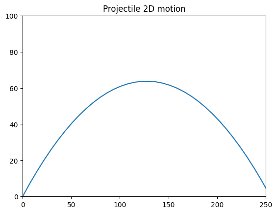
Lastly, remember that we can rewrite \(v_x\) and \(v_y\) in terms of \(\vec v\) using trigonometry. Thus, the general equation of projectile motion of an object launched at angle \(\theta_0\) and initial velocity \(\vec v_0\) is:

\[ x(t) = \vec v_0 \cos \theta_0 t \]

\[ y(t) = \vec v_0 \sin \theta_0 t - \frac{1}{2} gt^2 \]

A plot of the equation shows that it is correct:

import matplotlib.pyplot as plt
import numpy as np
from matplotlib.colors import LinearSegmentedColormap

t = np.linspace(0, 10)
v0 = 50
theta0 = np.pi / 4 # 45 degrees
g = 9.81
x = v0 * np.cos(theta0) * t
y = v0 * np.sin(theta0) * t - (1/2) * 9.81 * (t ** 2)

plt.plot(x, y)
plt.title("Projectile 2D motion")
plt.xlim(0, 250)
plt.ylim(0, 100)
plt.show()

Newton’s Laws

In the late-1600s, Isaac Newton came up with a series of 3 laws to describe a more general set of moving objects, not limited to objects in freefall. These form the foundation of Newtonian physics.

Newton’s 1st law states that objects in constant motion remain in motion unless acted on by a net force. A net force occurs when the forces acting on an object are not balanced. This means that objects in constant motion can have forces acting on them, but no net force, because all the forces are balanced.

Newton’s 2nd law states that a net force acts on an object to accelerate it, or mathematically:

\[ F_{net} = \sum F = ma \]

Newton’s 2nd law is often called the equation of motion for an object. To see why, notice that the law can be rewritten as:

\[ a = \frac{F_{net}}{m} \]

And since acceleration is the second derivative of position, this can be written:

\[ \frac{d^2 x}{dt^2} = \frac{F_{net}}{m} \]

Thus, solving for Newton’s second law gives the function \(x(t)\) that describes the motion of an object through space and time.

Newton’s 3rd law states that for every action force, there is an equal and opposite reaction force opposing it.

Of all of Newton’s laws, it is the second that is the most typically helpful.

To utilize Newton’s 2nd law, we often like to draw free-body diagrams to illustrate all the forces on an object. Forces that are in the positive direction (usually up and right) are positive, and forces in the negative direction (usually down and left) are negative. For instance, consider a free-falling object, influenced only by the downward force of gravity:

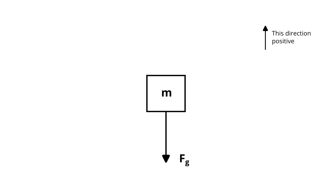
To apply Newton’s 2nd law, we first sum all the forces to find the net force:

\[ F_{net} = \sum F = 0 + (-F_g) = -F_g \]

Then, we equate the net force to \(ma\):

\[ F_{net} = ma \]

\[ -F_g = ma \]

Given that the force of gravity close to Earth is given by \(F_g = mg\), we can rewrite the last equation as:

\[ -mg = ma \]

Which we can simplify to:

\[ -g = a \]

To find the motion of the object, we need to recall that the acceleration is the second derivative of position, so:

\[ -g = \frac{d^2 s}{dt^2} \]

We can solve this differential equation by integrating both sides twice, to get:

\[ s(t) = v_0 t - \frac{1}{2}gt^2 + h_0 \]

A more difficult example is with the following system, where \(F_T\) is the tension force, transmitted by the rope:

Here, to draw a free-body diagram, we “unwrap” and stretch out the system, then draw 2 separate free-body diagrams for each sub-system:

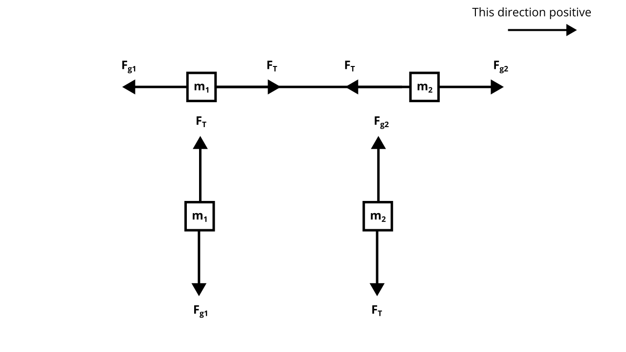
From there we can apply the 2nd law individually to each system. For the first system:

\[ \sum F = F_T + (-F_{g_1}) = m_1 a \]

Which we simplify to:

\[ F_T - F_{g_1} = m_1 a \]

And recalling \(F_g = mg\), we can further simplify with:

\[ F_T - m_1 g = m_1 a \]

And for the second system:

\[ \sum F = F_{g_2} + (-F_T) = m_2 a \]

Which we can simplify to:

\[ F_{g_2} -F_T = m_2 a \]

Again, we can use \(F_g = mg\) to further simplify with:

\[ m_2 g - F_T = m_2 a \]

We now have a simultaneous series of equations:

\[ F_T - m_1 g = m_1 a \]

\[ m_2 g - F_T = m_2 a \]

Solving them allows us to find the net acceleration of both systems:

\[ m_2 g - F_T = m_2 a \]

\[ m_2 g = F_T + m_2 a \]

\[ F_T = m_2 g - m_2 a \]

\[ F_T = m_1 a + m_1 g \]

\[ m_2 g - m_2 a = m_1 a + m_1 g \]

\[ m_2 g - m_1 g = m_1 a + m_2 a \]

\[ g(m_2 - m_1) = a(m_1 + m_2) \]

\[ a = \frac{g(m_2 - m_1)}{m_1 + m_2} \]

We can also use the same equations to derive a value of the tension force:

\[ F_T = \frac{2 m_1 m_2 g}{m_1 + m_2} \]

And the equation of motion for the entire system can be found by solving the differential equation, which is in turn found by substituting \(a\) for the second derivative of position:

\[ \frac{d^2 s}{dt^2} = \frac{g(m_2 - m_1)}{m_1 + m_2} \]

Using Newton’s laws usually results in a second-order differential equation for a system - one typically not easily solved, and usually only solvable via computer.

Finally, it is worth mentioning Newton’s law of universal gravitation, which states the gravitational force between two arbitrary distant masses (as opposed to close to Earth for \(F_g = mg\)) is given by:

\[ F_g = -\frac{G Mm}{r^2} \]

Where \(G\) is the universal gravitational constant, and \(G \approx 6.67 \times 10^{-11}\)

Work, Energy, and Power

Analyzing forces is one very good approach to finding the equations of motion for a system, but it has its drawbacks - the vector equation \(F_{net} = ma\) is often long and tedious to solve for. Another approach - the work-energy approach - is often much easier and more helpful for arriving at a solution when analyzing a given system.

At its simplest, work is simply force exerted over a distance:

\[ W = \int_{x_1}^{x_2} F dx \]

Kinetic energy \(K\), the energy of moving objects, is equal to the work done to accelerate an object from rest to a velocity \(v\). That is:

\[ K = \int_{x_1}^{x_2} F dx = \int_{x_1}^{x_2} ma dx = \int_{x_1}^{x_2} m \frac{dv}{dt} dx \]

Using the chain rule to expand out \(\frac{dv}{dt} = \frac{dv}{dx} \frac{dx}{dt}\), we have:

\[ \int_{x_1}^{x_2} m \frac{dv}{dx}\frac{dx}{dt} dx \]

If we move around the terms and rewrite \(\frac{dx}{dt} = v\), we get:

\[ \int_{x_1}^{x_2} m v \frac{dv}{dx} dx \]

The two \(dx\)’s cancel and as part of our substitution we replace our endpoints in \(x\) with endpoints in \(v\) to get:

\[ \int_0^v mv dv = \frac{1}{2} mv^2 \]

So:

\[ K = \frac{1}{2} mv^2 \]

For instance, a 1 kg object moving at \(10 \mathrm{\ m/s}\) will have a kinetic energy of 50 Joules.

Potential energy \(U\), the energy possessed by objects due to their position or configuration, is given by:

\[ U(x) = -W = -\int F dx \]

Attention

Note that the second equation (the integral of force with respect to position) only holds true for conservative forces in the single-variable case, where the work done is independent of the path taken.

For gravity, this results in:

\[ U_g (r) = -\int - \frac{G m_1 m_2}{r^2} dr = -\frac{G Mm}{r} \]

Note that an approximation for gravitational potential energy is \(U_g = mgh\), which works close to Earth.

For springs, where the elastic force is given by \(F = -kx\), this results in:

\[ U_s(x) = -\int -kx dx = \frac{1}{2} kx^2 \]

For electrostatics, where the electrostatic force is given by \(F = \frac{kq_1 q_2}{r^2}\), this results in:

\[ U_e (r) = -\int \frac{kq_1 q_2}{r^2} dr = \frac{kq_1 q_2}{r} \]

The potential energy, when expressed as a quantity, is always taken relative some reference point. For a falling object, a common reference point is the surface of the Earth. This means that on the Earth’s surface, an object has zero potential energy, while far from the Earth’s surface, the object has maximal potential energy.

The conservation of energy states that the sum of potential and kinetic energy is constant - that is, the sum of inital potential and kinetic energy is equal to the sum of final kinetic potential and kinetic energy:

\[ K_i + U_i = K_f + U_f \]

For example, let’s use the same cliff example as earlier, with the only difference being that we know that the final velocity of the falling object is \(48.9\mathrm{\ m/s}\).

Using the conservation of energy, we know that \(K_i = 0\) (as the object is thrown from rest), and \(U_f = 0\) (as the object is on the surface of the Earth, our reference point). So:

\[ U_i = K_f \]

\[ mgh = \frac{1}{2} m (v_f)^2 \]

\[ h = \frac{1}{2} \frac{m(v_f)^2}{g} \]

Plugging in the values, this gives us the same answer of the height of the cliff: 122 meters! However, note that we didn’t need to use any kinematic formulas, just an understanding of work and energy!

Momentum

Momentum is the product of mass and velocity:

\[ p = mv \]

Which also makes the derivative of the momentum force:

\[ F = \frac{dp}{dt} \]

And the (time) integral of force momentum:

\[ p = \int F dt \]

Do not confuse this with potential energy, which is the position integral of force!

Momentum cannot be created nor destroyed; it can only be transferred between objects. This is the principle of the conservation of momentum:

\[ P_{A_i} + P_{B_i} = P_{A_i} + P_{B_f} \]

Or more generally:

\[ \sum P_i = \sum P_f \]

Impulse is the change in momentum:

\[ J = \Delta P = \int_{t_1}^{t_2} F dt \]

Fields

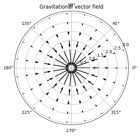
A vector field is an object that spans all of space and assigns a value to each point in space. For example, take the gravitational field, which gives each point a vector that is given by:

\[ \vec g(r) = \frac{GM}{r^2} \]

Here is a visualization of the gravitational field \(\vec g(r)\):

def plot_gfield():
    """
    Plot vector field of gravity in polar coordinates
    """
    G = 1
    M = 1
    radii = np.linspace(1, 3, 5)
    thetas = np.linspace(0, 2 * np.pi, 20)
    theta, r = np.meshgrid(thetas, radii)
    R = -(G * M) / (r ** 2)

    f = plt.figure()
    ax = f.add_subplot(polar=True)
    ax.quiver(theta, r, R * np.cos(theta), R * np.sin(theta))
    plt.title("Gravitational vector field")
    plt.show()

plot_gfield()

The gravitational field is related to the gravitational force by:

\[ \vec g = \frac{F}{m} \]

That means that at each point in the field, an object of mass \(m\) will feel a force of \(\vec g m\).

A potential field, similar to a vector field, is an object that spans all of space and assigns a scalar to each point in space. Potentials have the special property that their slopes are equal to another vector field. For example, the gravitational (vector) field \(\vec g\) is related to the gravitational potential \(\phi\) by:

\[ \vec g = - \nabla \phi = -\left( \frac{\partial \phi}{\partial x}, \frac{\partial \phi}{\partial y}, \frac{\partial \phi}{\partial z} \right) \]

From this, we can derive that the gravitational potential is given by:

\[ \phi = \frac{GM}{r} \]

A visualization of the gravitational potential is shown below:

def calc_div_grav():
    %matplotlib inline
    G = 1
    M = 1
    radii = np.linspace(0.4, 7, 50)
    thetas = np.linspace(0, 2 * np.pi, 50)
    R, T = np.meshgrid(radii, thetas)
    Phi = -(G * M)/(R)
    
    # convert r, theta coordinates to
    # cartesian x, y coordinates
    X, Y = R*np.cos(T), R*np.sin(T)
    
    f = plt.figure(figsize=(7, 7))
    ax = f.add_subplot(projection="3d")
    # Set the angle of the camera
    ax.view_init(25, -45)
    ax.set_zlim(-3, 3)
    
    # Colormap
    cmap = LinearSegmentedColormap.from_list("", ["#D54C90", "#A37DF8", "#B3E6FF"])
    ax.plot_surface(X, Y, Phi,linewidth=0.1 ,
                    cmap=cmap,
                    alpha=1,
                    cstride=2,
                    rstride=2,
                    edgecolors="black")
    plt.title("Gravitational potential field $\Phi$")
    plt.grid()
    plt.rcParams["figure.autolayout"] 
    plt.show()

calc_div_grav()

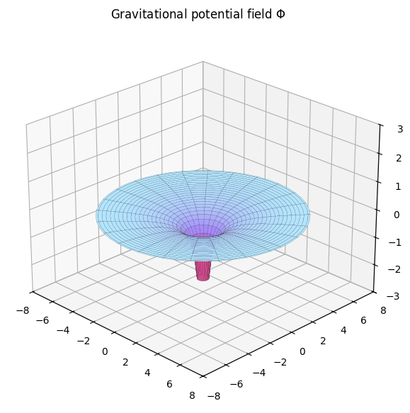
The gravitational potential is related to the gravitational potential energy by:

\[ \phi = \frac{U}{m} \]

That means that at each point in the potential field, an object of mass \(m\) will have a gravitational potential energy of \(\phi m\) relative to infinity.

The divergence of the gravitational field is given by:

\[ \nabla \cdot \vec g = -4\pi G \rho \]

Combining the two equations, we can find the gravitational potential in terms of its mass density:

\[ \vec g = - \nabla \Phi \]

\[ \nabla \cdot - \nabla \Phi = \nabla^2 \Phi = 4 \pi G \rho \]

This is Poisson’s equation:

\[ \nabla^2 \Phi = 4 \pi G \rho \]

In empty space, the equation reduces to:

\[ \nabla^2 \Phi = 0 \]