Linear Algebra

A vector is a list of items (usually numbers), which represent coordinates in a certain coordinate system. For example, the vector \((4, 2)\) is a line that moves 4 in the x-direction, and 2 in the y-direction. We draw vectors as arrows in space.

A scalar is a number that “scales” (that is, shrinks or stretches) a vector. More generally, a scalar is any singular number.

To write a vector (say, \(\vec a\)), we have several notations:

\[\begin{split} \vec a = (4, 2) = \begin{bmatrix} 4 \\ 2 \end{bmatrix} = 4 \hat i + 2 \hat j \end{split}\]

The first (point notation) is used for both points and vectors and is the simplest method. The second (matrix notation) is the same thing, just written out vertically in a column. The third (basis vector notation) is slightly different. It defines a vector as a sum of transformed basis vectors, where:

\[\begin{split} \hat i = \begin{bmatrix} 1 \\ 0 \\ 0 \end{bmatrix}, \hat j = \begin{bmatrix} 0 \\ 1 \\ 0 \end{bmatrix}, \hat k = \begin{bmatrix} 0 \\ 0 \\ 1 \end{bmatrix} \end{split}\]

The basis vectors are then used to “construct” a vector like this:

Note

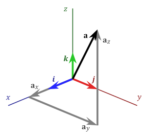
A basis vector can be thought of as a vector with a “tail” at the origin and a “head” at 1 unit from the origin along one of the axes.

We can then express any vector as a linear combination of the basis vectors:

\[ \vec a = s_1 \hat i + s_2 \hat j + s_3 \hat k \]

Note

A linear combination of basis vectors simply means that we stretch or shrink each basis vector by a certain factor (\(s\) being that factor), and then add those stretched/shrinked vectors together to form the final vector.

We use the basis vectors \(\hat i, \hat j, \hat k\) in 2D and 3D space, but for nth-dimensional spaces, we use the more general basis vectors \(e_1, e_2, e_3, \dots e_n\), so linear combinations work like this:

\[ \vec a = s_1 \vec e_1 + s_2 \vec e_2 + s_3 \vec e_3 + \dots + s_n \vec e_n \]

Which we often write as:

\[ \vec a = \sum_{i = 1}^n s_i \vec e_i \]

Important

Remember this notation! This will be very important later on.

To add vectors of any dimension, we add their corresponding components:

\[\begin{split} \begin{bmatrix} a_1 \\ a_2 \\ a_3 \end{bmatrix} + \begin{bmatrix} b_1 \\ b_2 \\ b_3 \end{bmatrix} = \begin{bmatrix} a_1 + b_1 \\ a_2 + b_2 \\ a_3 + b_3 \end{bmatrix} \end{split}\]

To multiply a vector by a scalar, we multiply the scalar by each of the components:

\[\begin{split} k \begin{bmatrix} a_1 \\ a_2 \\ a_3 \end{bmatrix} = \begin{bmatrix} k (a_1) \\ k (a_2) \\ k (a_3) \end{bmatrix} \end{split}\]

To find the length of a vector, we take its magnitude, like this:

\[ \operatorname{magn}(\vec a) \]

A note on notation

You will also see the magnitude of a vector written as \(||\vec a||\) but I highly recommend not using this alternate notation, because it is so easily confused with the absolute value symbol.

The magnitude of a vector can be found using the Pythagorean theorem, so the magnitude is the square of the sum of each component:

\[\begin{split} \operatorname{magn} \: \begin{bmatrix} a_1 \\ a_2 \\ a_3 \\ \dots \\ a_n \end{bmatrix} = \sqrt{(a_1)^2 + (a_2)^2 + (a_3)^2 + \dots + (a_n)^2} \end{split}\]

The dot product (or inner product) between vectors tells us how much 2 vectors point in the same direction. The dot product is usually defined like this:

\[ \vec a \cdot \vec b = \operatorname{magn}(\vec a) \operatorname{magn}(\vec b) \cos (\theta) \]

The more two vectors point in the same direction, the larger the dot product, and vice-versa. If the dot product is zero, that means the vectors are perpendicular to each other, and if the dot product is negative, that means the vectors are pointing in opposite directions.

The dot product returns a scalar, and there is a simpler formula for computing it:

\[\begin{split} \begin{bmatrix} a_1 \\ a_2 \\ a_3 \end{bmatrix} \cdot \begin{bmatrix} b_1 \\ b_2 \\ b_3 \end{bmatrix} = \begin{bmatrix} a_1 \cdot b_1 \\ a_2 \cdot b_2 \\ a_3 \cdot b_3 \end{bmatrix} \end{split}\]

The cross product between vectors returns a new vector perpendicular to both vectors with a magnitude proportional to how far apart the two vectors are pointing. The cross product is usually written like this:

\[ \vec a \times \vec b \]

And the magnitude of the cross product is this:

\[ \operatorname{mag} (\vec a \times \vec b) = \operatorname{magn}(\vec a) \operatorname{magn}(\vec b) \sin (\theta) \]

The cross product can be calculated by writing a special matrix that looks like this:

\[\begin{split} \begin{vmatrix} \hat i & \hat j & \hat k \\ a_1 & a_2 & a_3 \\ b_1 & b_2 & b_3 \end{vmatrix} \end{split}\]

Now, we compute each component of the cross product vector by blocking out the column under that component’s basis vector in that matrix. For example, for \(\hat i\), we block out the first column under it:

\[\begin{split} \begin{vmatrix} \hat i & \hat j & \hat k \\ \Box & a_2 & a_3 \\ \Box & b_2 & b_3 \end{vmatrix} \end{split}\]

This leaves us with a square matrix underneath the basis vectors. We just need to compute a special value called the determinant of that matrix, which is given by:

\[\begin{split} \begin{vmatrix} a & b \\ c & d \end{vmatrix} = ad - bc \end{split}\]

In our case, we have:

\[\begin{split} \begin{vmatrix} a_2 & a_3 \\ b_2 & b_3 \end{vmatrix} = a_2 b_3 - a_3 b_2 \end{split}\]

We do the same for all three basis vectors, which gives us this:

\[\begin{split} \vec a \times \vec b = \begin{vmatrix} \hat i & \hat j & \hat k \\ \Box & a_2 & a_3 \\ \Box & b_2 & b_3 \end{vmatrix} - \begin{vmatrix} \hat i & \hat j & \hat k \\ a_1 & \Box & a_3 \\ b_1 & \Box & b_3 \end{vmatrix} + \begin{vmatrix} \hat i & \hat j & \hat k \\ a_1 & a_2 & \Box \\ b_1 & b_2 & \Box \end{vmatrix} \end{split}\]

\[\begin{split} \vec a \times \vec b = \begin{vmatrix} a_2 & a_3 \\ b_2 & b_3 \end{vmatrix} \hat i - \begin{vmatrix} a_1 & a_3 \\ b_1 & b_3 \end{vmatrix} \hat j + \begin{vmatrix} a_1 & a_2 \\ b_1 & b_2 \end{vmatrix} \hat k \end{split}\]

\[ \vec a \times \vec b = (a_2 b_3 - a_3 b_2)\hat i - (a_1 b_3 - a_3 b_1)\hat j + (a_1 b_2 - a_2 b_1)\hat k \]

Note

Be careful, remember that it is the first determinant times \(\hat i\), then minus the second determinant times \(\hat j\), and then plus the third determinant times \(\hat k\).

A matrix is an array of items (usually numbers), arranged in rows and columns. The dimension of a matrix is how many rows and columns it has. A two-by-three \((2 \times 3)\) matrix, for example, has two rows and 3 columns, like this:

\[\begin{split} A = \begin{pmatrix} 1 & 2 & 3 \\ 4 & 2 & 1 \end{pmatrix} \end{split}\]

We denote the rows of the matrix typically with the letter \(i\), and the columns with the letter \(j\), and we can refer to the entries of a matrix with their column and row number. For example, \(A_{2 3}\) is the entry on the 2nd row, 3rd column of the matrix \(A\).

A matrix can be n-dimensional. A higher-dimensional matrix with \(i\) rows and \(j\) columns would be written like this:

\[\begin{split} A = \begin{pmatrix} A_{11} & A_{12} & A_{13} & \dots & A_{1j} \\ A_{21} & A_{22} & A_{23} & \dots & A_{2j} \\ \vdots & \vdots & \vdots & \ddots & \vdots \\ A_{i1} & A_{i2} & A_{i3} & \dots & A_{ij} \\ \end{pmatrix} \end{split}\]

The transpose of a matrix is the matrix with its rows and columns switched, such that:

\[ (A_{ij})^T = A_{ji} \]

We can write out a vector as a row vector or column vector, which are respectively matrices with just one row or column:

\[\begin{split} \vec a = \begin{bmatrix} a_1 & a_2 & a_3 \end{bmatrix}^T = \begin{bmatrix} a_1 \\ a_2 \\ a_3 \end{bmatrix} \end{split}\]

Important

Note that while a vector can be arbitrarily written as a row or column vector, a row vector is not the same thing as a column vector!

A matrix is a description of a linear transformation of the grid. To understand what this means, let’s go back to our basis vectors for a moment. Remember that (in 2D space), the basis vectors \(\hat i\) and \(\hat j\) are:

\[\begin{split} \hat i = \begin{bmatrix} 1 \\ 0 \end{bmatrix}, \hat j = \begin{bmatrix} 0 \\ 1 \end{bmatrix} \end{split}\]

Now, suppose we had a matrix \(A\), as follows:

\[\begin{split} A = \begin{bmatrix} 2 & 1 \\ 5 & 1 \end{bmatrix} \end{split}\]

This matrix tells us to move the basis vectors \(\hat i\) and \(\hat j\) like this:

\[\begin{split} \hat i: \begin{bmatrix} 1 \\ 0 \end{bmatrix} \rightarrow \begin{bmatrix} 2 \\ 5 \end{bmatrix} \end{split}\]

\[\begin{split} \hat j: \begin{bmatrix} 0 \\ 1 \end{bmatrix} \rightarrow \begin{bmatrix} 1 \\ 1 \end{bmatrix} \end{split}\]

By moving the basis vectors, every other point on our original grid moves too, so every vector on the original grid moves with it. So, a matrix is a way to transform vectors into new positions by changing the entire grid.

Matrix Operations

We can add matrices together if they have the same dimensions:

\[\begin{split} \begin{bmatrix} A_{11} & A_{12} \\ A_{21} & A_{22} \end{bmatrix} + \begin{bmatrix} B_{11} & B_{12} \\ B_{21} & B_{22} \end{bmatrix} = \begin{bmatrix} A_{11} + B_{11} & A_{12} + B_{12} \\ A_{21} + B_{21} & A_{22} + B_{22} \end{bmatrix} \end{split}\]

We can multiply any matrix by a scalar:

\[\begin{split} k \begin{bmatrix} A_{11} & A_{12} \\ A_{21} & A_{22} \end{bmatrix} = \begin{bmatrix} k(A_{11}) & k(A_{12}) \\ k(A_{21}) & k(A_{22}) \end{bmatrix} \end{split}\]

And we can multiply matrices with other matrices. To do so, we calculate the dot product of each row vector of matrix \(A\) with each column vector of matrix \(B\).

In general, when finding the entry \(C_{ij}\) where \(C\) is the matrix product of \(A\) and \(B\), we take the dot product of the \(i\)th row of \(A\) with the \(j\)th column of \(B\).

This is a bit of a more multi-step process, so let’s see how this works, given our two example matrices \(A\) and \(B\) with the matrix product \(C\):

\[\begin{split} \begin{bmatrix} A_{11} & A_{12} \\ A_{21} & A_{22} \end{bmatrix} \begin{bmatrix} B_{11} & B_{12} \\ B_{21} & B_{22} \end{bmatrix} = \begin{bmatrix} C_{11} & C_{12} \\ C_{21} & C_{22} \end{bmatrix} \end{split}\]

First, we take the first row vector of \(A\) and multiply it by the first column vector of \(B\):

\[\begin{split} C_{11} = \begin{bmatrix} A_{11} & A_{12} \end{bmatrix} \cdot \begin{bmatrix} B_{11} \\ B_{12} \end{bmatrix} = A_{11} B_{11} + A_{12} B_{12} \end{split}\]

Then, we take the second row vector of \(A\) and multiply it by the same first column vector of \(B\):

\[\begin{split} C_{21} = \begin{bmatrix} A_{21} & A_{22} \end{bmatrix} \cdot \begin{bmatrix} B_{11} \\ B_{12} \end{bmatrix} = A_{21} B_{11} + A_{22} B_{12} \end{split}\]

If the first matrix had more rows, we’d keep doing this, until we’ve multiplied every row of the first matrix by the first column of the second matrix.

Now, we take the first row vector of \(A\) and multiply it by the second column vector of \(B\):

\[\begin{split} C_{12} = \begin{bmatrix} A_{11} & A_{12} \end{bmatrix} \cdot \begin{bmatrix} B_{12} \\ B_{22} \end{bmatrix} = A_{11} B_{12} + A_{12} B_{22} \end{split}\]

Then, we take the second row vector of \(A\) and multiply it by the same second column vector of \(B\):

\[\begin{split} C_{22} = \begin{bmatrix} A_{21} & A_{22} \end{bmatrix} \cdot \begin{bmatrix} B_{11} \\ B_{12} \end{bmatrix} = A_{21} B_{11} + A_{22} B_{12} \end{split}\]

We’d continue this process, going through all the columns of the second matrix. Putting it all together, we find the final matrix product.

Since matrix multiplication is dependent on the dot product, we can only multiply two matrices \(A\) and \(B\) if \(A\) has the same number of columns as \(B\) has rows. So we can find the matrix product of two \(3 \times 3\) matrices, or a \(5 \times 2\) matrix with a \(2 \times 5\) matrix, but not a \(5 \times 2\) and \(3 \times 3\) matrix.

Why is matrix multiplication useful? Well, because remember matrices are transformations that can be applied to vectors. If we want to apply two matrices, \(A\) and \(B\), to a vector \(\vec a\), that’s the same as transforming \(\vec a\) by the matrix product \(AB\).

Using matrices to transform vectors

We can use matrices to transform vectors as well, using a modified version of matrix multiplication. The general formula for matrix-vector multiplication is given by:

\[\begin{split} \begin{align*} A \vec x= \left[ \begin{array}{cccc} a_{11} & a_{12} & \ldots & a_{1n}\\ a_{21} & a_{22} & \ldots & a_{2n}\\ \vdots & \vdots & \ddots & \vdots\\ a_{m1} & a_{m2} & \ldots & a_{mn} \end{array} \right] \left[ \begin{array}{c} x_1\\ x_2\\ \vdots\\ x_n \end{array} \right] = \left[ \begin{array}{c} a_{11}x_1+a_{12}x_2 + \cdots + a_{1n} x_n\\ a_{21}x_1+a_{22}x_2 + \cdots + a_{2n} x_n\\ \vdots\\ a_{m1}x_1+a_{m2}x_2 + \cdots + a_{mn} x_n\\ \end{array} \right]. \end{align*} \end{split}\]

Consider the following matrix and vector:

\[\begin{split} S = \begin{bmatrix} 2 & 0 \\ 0 & 2 \end{bmatrix}, \vec v = \begin{bmatrix} 5 \\ 2 \end{bmatrix} \end{split}\]

If we apply the matrix \(S\) on a vector \(\vec v\), then we end up with a new vector \(\vec v_2\):

\[\begin{split} S \vec v = \begin{bmatrix} 2 & 0 \\ 0 & 2 \end{bmatrix} \cdot \begin{bmatrix} 5 \\ 2 \end{bmatrix} = \begin{bmatrix} 10 \\ 4 \end{bmatrix} \end{split}\]

We can check our answer using NumPy’s dot(), which performs matrix-vector multiplication when given a matrix and a vector:

import numpy as np

a = np.array([[2, 0], 
              [0, 2]])
b = np.array([[5], 
              [2]])
a.dot(b)

array([[10],
       [ 4]])

Note that the new vector \(\vec v_2\) is equal to the original vector \(\vec v_1\) scaled by 2! So the matrix \(S\) actually encodes the linear transformation of scaling by 2. In fact, all matrices can be thought of as linear maps that map vectors onto their transformed versions. Common transformations, such as rotation, shearing, stretching, translation, and countless others can all be encoded through matrices! This is why matrices are useful!

Linearity

Linear algebra might seem an unrelated mess of mathematical objects, problems, and techniques. But there is one theme underlying linear algebra - linearity. Anything that is linear is acted on by linear operators, to which the following rule applies:

\[ f(ax + by) = af(x) + bf(y) \]

For example, one linear operator would be vector addition, and another linear operator would be matrix multiplication - both follow this rule. Therefore vectors and matrices are linear as well.

What’s the point?

Linear algebra has many arbitrary rules - but why learn them? What does linear algebra have to do with the real world, when it feels like you’re just moving around a bunch of numbers in columns and rows? The answer is - a lot.

For example, matrices are used to solve complicated systems of equations, and find optimal solutions to many problems. Vectors are used to model physical quantities, like force, position, and acceleration. Almost all computer graphics and machine learning uses both, and physics uses both in combination with other mathematics. In fact, the whole reason why linear algebra is called linear algebra is that it provides a consistent set of rules that apply to linear problems. Put it another way, any linear problem can be solved with linear algebra!

Extra: motivation for tensors

Consider a 3D vector:

\[\begin{split} \vec A = \begin{bmatrix} x \\ y \\ z \end{bmatrix} = \begin{bmatrix} 3 \\ -5 \\ 2 \end{bmatrix} \end{split}\]

This vector is written in Cartesian coordinates (x, y, z coordinates). The same vector would be written like this in spherical coordinates (\(\theta\) and \(\phi\) are given in radians):

\[\begin{split} \vec A = \begin{bmatrix} r \\ \theta \\ \phi \end{bmatrix} = \begin{bmatrix} (x^2 + y^2 + z^2)^{1/2} \\ \arctan (y/x) \\ \arccos (z^2/(x^2 + y^2 + z^2)) \end{bmatrix} = \begin{bmatrix} 6.164 \\ -1.03 \\ 0.324 \end{bmatrix} \end{split}\]

Notice that these two are the same vector, but in different coordinate systems, the components of the vector change. So, a vector’s components are not invariant. They depend on the coordinate system you use, and converting between coordinate systems is really annoying!

This is where tensors come in. Tensors are generalizations of n-dimensional arrays - including vectors and matrices - which are invariant. This means, we can rewrite a scalar, vector, or matrix as an equivalent tensor that remains the same in whichever coordinate system we put it in. How cool is that! We’ll explore tensors some more a few sections later.