Special Relativity

“Henceforth space by itself, and time by itself, are doomed to fade away into mere shadows, and only a kind of union of the two will preserve an independent reality…”

Hermann Minkowski (1908)

For over 200 years, the basic premises of Newtonian mechanics remained absolute. Space and time were separate entities, and the laws of physics followed Newton’s postulates. That is, until 1905, when Einstein broke both previously-assumed absolute truths, and set out to create a new theory. This groundbreaking theory was the theory of Special Relativity, a description of the motion of objects that supercedes Newtonian mechanics and completely revolutionized our understanding of the world.

import matplotlib.pyplot as plt
import numpy as np

Events

An event is anything that happens that can be measured. This can be a rocket flying through your window, a book that falls on your head, a crater that opens in your room, or all three at once! We can describe events with coordinates - perhaps your rocket-falling-book-crater event happened at position 3 meters to your right, 2 meters to your front, and 0 meters above your head, at time 2:55pm. Physicists obsess over events, because everything in physics is composed of a sequence of events, and so using the laws of physics, physicists can predict what events will happen.

Galilean Relativity

Imagine you were seated aboard a train, and the train was moving with constant velocity. Are you moving and the earth underneath you stationary? Or is the train stationary and the earth is moving under you? In physics, both of these interpretations can be true - your understanding of your motion must be considered relative to some other object. For instance, you can pick the stationary object to be the earth, in which case you would be considered moving, or you could pick the stationary object to be yourself on the train, in which case the Earth would be moving. In either case, the laws of physics remain the same.

Reference frames

A reference frame is a coordinate system with an origin centered at a chosen location. For example, you can choose your origin to be a house on the surface of the Earth, a moving train, a rocket, even a random point in interstellar space. You would then have a reference frame at that origin.

Typically speaking, however, when we refer to the reference frame of an observer, the origin is located at wherever the observer is located. So the reference frame of an astronaut in a rocket would have an origin centered at that rocket. In the astronaut’s reference frame, they themselves are located at the point \((0, 0, 0)\), and everything else (such as the motion of the Earth) is measured relative to them.

We use reference frames to measure everything around us, everything from the position and velocities of objects to forces between objects. In fact, without reference frames, we wouldn’t be able to measure any motion at all.

Transformations

In physics, it is sometimes easier to do calculations in one reference frame than another - no one would like to compute the trajectory of a baseball on Earth from the reference frame of another galaxy! So, we want to be able to convert measurements from one reference frame to another.

The reference frame of an observer is known as the unprimed frame. The observer is at rest with respect to the unprimed frame, and everything is moving relative to them. Any measurement in the unprimed frame is described by coordinates \((t, x, y, z)\).

Everything moving relative to the observer has a reference frame of its own. For example, our astronaut could be observing Earth, the Sun, the Moon, a space station - and each of those objects has its own reference frame. The observer measures the velocity \(v\) at which each reference frame moves with respect to the observer. These other moving reference frames are known as primed frames because they are denoted with the prime (\('\)) symbol. Any measurement in a primed frame is described by the coordinates \((t', x', y', z')\).

These sets of different measurements are related as follows:

\[ x' = x - vt \]

\[ y' = y \]

\[ z' = z \]

\[ t' = t \]

Note

The primes here are not derivative symbols, they’re used in this context to denote “different” or “alternate”

One thing we specifically notice is that here, time is absolute - the same in every reference frame. As we will see, this will no longer hold true in special relativity.

The constant speed of light

In the late 19th-century, physicists finally came up with one unified theory of electromagnetism using Maxwell’s equations, which we saw earlier. Recall that the equations are given by:

\[ \nabla \cdot \vec E = \frac{\rho}{\epsilon_0} \]

\[ \nabla \times \vec E = -\frac{\partial \vec B}{\partial t} \]

\[ \nabla \cdot \vec B = 0 \]

\[ \nabla \times \vec B = \mu_0 \vec J + \mu_0 \epsilon_0 \frac{\partial \vec E}{\partial t} \]

Let’s take Faraday’s law:

\[ \nabla \times \vec E = -\frac{\partial \vec B}{\partial t} \]

Suppose we take the curl of both sides:

\[ \nabla \times (\nabla \times \vec E) = \nabla \times -\frac{\partial \vec B}{\partial t} \]

The right hand side can be rearranged to be:

\[ \nabla \times (\nabla \times \vec E) = -\frac{\partial}{\partial t} (\nabla \times \vec B) \]

Which simplifies to:

\[ \nabla \times (\nabla \times \vec E) = -\mu_0 \epsilon_0 \frac{\partial^2 \vec E}{\partial t^2} \]

We can use the vector identity \(\nabla \times (\nabla \times \vec E) = -\nabla^2 E\) to simplify further to:

\[ \nabla^2 E = \mu_0 \epsilon_0 \frac{\partial^2 \vec E}{\partial t^2} \]

Using the same technique for Ampére’s law and then Faraday’s law yields the same result for magnetic fields:

\[ \nabla^2 B = \mu_0 \epsilon_0 \frac{\partial^2 \vec B}{\partial t^2} \]

Note that this looks very much like the wave equation:

\[ \nabla^2 f = \frac{1}{v^2} \frac{\partial^2 f}{\partial t^2} \]

Which means that oscillating electric and magnetic fields produce electromagnetic waves that move through space at a speed \(v\). We can solve for \(v\) by noting that:

\[ \frac{1}{v^2} = \mu_0 \epsilon_0 \]

This yields:

\[ v = \frac{1}{\sqrt{\mu_0 \epsilon_0}} = 299792458 \mathrm{\ m/s} = c \]

Now notice something special. The velocity \(c\) of electromagnetic waves - light waves - is a constant, because it is composed of the reciprocal of the square root of two other constants. This means that regardless of the velocity of the reference frame, it must be the same speed.

However, remember that in Galilean relativity, we defined that velocities add by \(\vec v + \vec u\). So we’d expect that an observer in a moving reference frame would measure a higher speed of light, while observers in a stationary reference frame would measure a lower speed of light. Through numerous experiments, this was proven not to be the case - we are certain that the speed of light is constant, regardless of the reference frame.

Therefore, the Galilean transformations must be wrong, and a new set of transformations - the Lorentz transformations - must supercede them.

The Lorentz Transformations

The Lorentz transformations are Einstein’s revision to Galilean relavity, derived from two postulates:

• The laws of physics hold true in every reference frame

• The speed of light \(c\) is constant in every reference frame

To derive the Lorentz transformations, let’s start with the Galilean transformations for \(x \rightarrow x'\) and \(x' \rightarrow x\):

\[ x' = x - vt \]

\[ x = x' + vt' \]

To correct Galilean coordinate transformations, we intuitively need to multiply the Galilean transformations by a factor \(\gamma\), which we can think of as the “correcting factor” to make sure that the Galilean transforms preserve the speed of light in every reference frame:

\[ x' = \gamma (x - vt) \]

\[ x = \gamma (x' + vt') \]

Now, we can multiply the left and right hand sides of the equation together, to combine the two equations into one equation:

\[ x' x = \gamma (x - vt) \gamma (x' + vt') \]

\[ x' x = \gamma^2 (xx' + xvt - x'vt - v^2 t t') \]

Remember the second postulate of special relativity is that the speed of light is an invariant in every reference frame - that is \(c = \frac{x}{t} = \frac{x'}{t'}\). Rearranging, we can say that \(x = ct\) and \(x' = ct'\). Substituting that in, we have:

\[ c^2 tt' = \gamma^2 (c^2 tt' + ct vt - ct' vt - v^2 tt') \]

The two middle terms cancel each other out, so we have:

\[ c^2 tt' = \gamma^2 (c^2 tt' - v^2 tt') \]

We isolate \(\gamma^2\) by dividing the right-hand side of the equation by the left, to obtain:

\[ \gamma^2 = \frac{c^2 tt'}{c^2 tt' - v^2 tt'} \]

We can factor out the common factor of \(tt'\), to get:

\[ \gamma^2 = \frac{c^2 tt'}{tt'(c^2 - v^2)} \]

\[ \gamma^2 = \frac{c^2}{(c^2 - v^2)} \]

We can then simplify by dividing both the numerator and denominator by \(c^2\), which gives us:

\[ \gamma^2 = \frac{1}{1 - \frac{v^2}{c^2}} \]

\[ \gamma^2 = \frac{1}{1 - \left(\frac{v}{c}\right)^2} \]

Finally, taking the square root, we have:

\[ \gamma = \frac{1}{\sqrt{1 - \left(\frac{v}{c}\right)^2}} \]

We can use this to derive the Lorentz transformations for \(x\), \(y\), and \(z\), but we need a little more algebra to figure out the Lorentz transform for \(t\). To do this, we first write out the Lorentz transformations from \(x \rightarrow x'\) and \(x' \rightarrow x\):

\[ x' = \gamma(x - vt) \]

\[ x = \gamma (x' + vt') \]

We take the second equation to solve for \(t'\):

\[ t' = \frac{x}{\gamma v} - \frac{x'}{v} \]

And we can now plug in the first Lorentz transformation equation into \(x'\):

\[ t' = \frac{x}{\gamma v} - \frac{\gamma(x - vt)}{v} \]

We can now distribute to find:

\[ t' = \gamma \left(\frac{x}{\gamma^2 v} - \frac{x}{v} + t\right) \]

We can further factor out the first two terms as:

\[ t' = \gamma \left(x\left[\frac{1}{\gamma^2 v} - \frac{1}{v}\right]+ t\right) \]

This simplifies to:

\[ t' = \gamma \left(x\left[\frac{1- \gamma^2}{\gamma^2 v}\right] + t\right) \]

Which then simplifies to:

\[ t' = \gamma \left(-\frac{xv}{c^2} + t\right) \]

Or:

\[ t' = \gamma \left(t - \frac{vx}{c^2}\right) \]

So, we now have the complete set of Lorentz transformations, which obey the laws of special relativity:

\[ t' = \gamma \left(t - \frac{vx}{c^2}\right) \]

\[ x' = \gamma (x - vt) \]

\[ y' = y \]

\[ z' = z \]

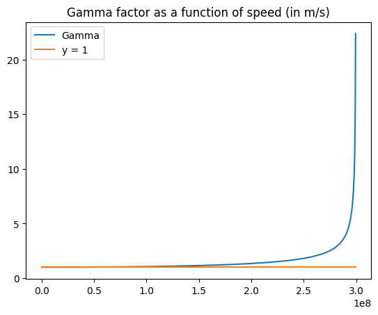
Where the Lorentz factor \(\gamma\) is approximately 1 at speeds of everyday life, but rises to infinity as you approach \(c\):

c = 299792458
v = np.linspace(0, 0.999 * c, 1000)
gamma = 1 / np.sqrt(1 - (v / c) ** 2)
one = np.ones(len(v))

plt.plot(v, gamma, label="Gamma")
plt.plot(v, one, label="y = 1")
plt.legend()
plt.title("Gamma factor as a function of speed (in m/s)")
plt.show()

The idea of spacetime

In classical physics, time had always been thought of as a steady feature in the background of the universe, something that was universal, and crucially, experienced the same way by everyone. But now, with the Lorentz transforms, it was clear that time was a dimension, like any other, and it couldn’t be separated from the dimensions of space. Hence, the new idea of spacetime was born - a 4-dimensional space that contained space and time.

But how would this new spacetime be described? One way to describe spacetime is by defining a metric, which we saw back in tensor calculus. A metric can be used to define how distances are measured in space. For instance, in 2D Euclidean space, we can measure distances with:

\[ ds^2 = dx^2 + dy^2 \]

which is just the Pythagorean theorem. Hermann Minkowski, Einstein’s former professor, recognized that this metric would not work in special relativity when applied to spacetime. He instead proposed a different metric, which we today know as the Minkowski metric.

We start from the Euclidean metric in three dimensions:

\[ ds^2 = dx^2 + dy^2 + dz^2 \]

Now, if we add a time dimension, and still consider Euclidean space, we have:

\[ ds^2 = dt^2 + dx^2 + dy^2 + dz^2 \]

We want to use the same units for time as well as space (units of meters). Otherwise, we would have incompatible units in our metric. Thus, we add a factor of \(c^2\) to get:

\[ ds^2 = dt^2 + dx^2 + dy^2 + dz^2 \]

Now, note the observation that in special relativity, as an object moves faster, it experiences less time, instead of more time, as in Euclidean space. Therefore, the time component of the metric must be negative:

\[ ds^2 = -c^2 dt^2 + dx^2 + dy^2 + dz^2 \]

We have arrived at the Minkowski metric.

Consequences of special relativity

Relativity of simultaneity

Let’s go back to the Lorentz transform for time coordinates:

\[ t' = \gamma \left(t - \frac{vx}{c^2}\right) \]

We can rewrite this equation equivalently in terms of changes in time:

\[ \Delta t' = \gamma \left(\Delta t - \frac{v \Delta x}{c^2}\right) \]

From this equation, it is clear that two events with \(\Delta t = 0\) - happening simultaneously in one frame - do not necessarily imply that \(\Delta t' = 0\) - that is, they are happening simultaneously in the other frame. In fact, the actual case is that:

\[ \Delta t = 0 \Rightarrow \Delta t' = -\frac{\gamma v\Delta x}{c^2} \]

Which implies that events that are simultaneous in frame \(S\) are separated by a time of \(-\frac{\gamma v\Delta x}{c^2}\) in frame \(S'\). This is the relativity of simultaneity.

Time dilation

Again, we return to the equation:

\[ \Delta t' = \gamma \left(\Delta t - \frac{v \Delta x}{c^2}\right) \]

In this case, suppose we have two clocks, one at rest aboard a moving spaceship (frame \(S'\)), and one at rest on Earth (frame \(S\)). Because both clocks are not moving, we can say that \(\Delta x = 0\). But this leads us to find something strange:

\[ \Delta t' = \gamma \Delta t \]

That is, more time passes on Earth than aboard the spaceship during the same measured time interval. Or put it another way, clocks tick more slowly when placed in a moving reference frame. For instance, a 3-second time interval for a spaceship going at 80% light speed would be measured as 7-seconds by the earthbound clock. In practice, this effect doesn’t show up until a reference frame is moving at more than 50% of the speed of light, but in interstellar spaceflight, the effects can be dramatic - at 99.999% of the speed of light, one year aboard a spacecraft would be 223 years on Earth! In fact, this is one mode of time travel into the future - passengers aboard a very fast craft would experience little time, while a lot more time passes for stationary observers, allowing passengers to seemingly magically travel into the future.

Length contraction

We first take the x-coordinate Lorentz transform equation, and we write it in terms of the change in \(x\):

\[ \Delta x' = \gamma (\Delta x - v \Delta t) \]

We set \(\Delta t = 0\) as we want a snapshot of one moment in time - therefore, we have:

\[ \Delta x' = \gamma \Delta x \]

We can solve for \(\Delta x\) with:

\[ \Delta x = \frac{\Delta x'}{\gamma} \]

This means in the stationary frame, a moving object would be contracted along the direction of motion. This means in the paradoxical case that a meterstick travelling at 90% or more than the speed of light would be able to fit into a barn house less than a meter long.

Relativistic addition of velocities

\[ u'={\frac {dx'}{dt'}}={\frac {\gamma (dx-vdt)}{\gamma \left(dt-{\frac {vdx}{c^{2}}}\right)}}={\frac {{\frac {dx}{dt}}-v}{1-\left({\frac {v}{c^{2}}}\right)\left({\frac {dx}{dt}}\right)}}={\frac {u-v}{1-uv/c^{2}}} \]

Proper length and proper time:

Proper time \(\tau\) is the time measured by an observer’s own clock as the observer moves through spacetime. It is related to the coordinate time \(t\), which is the clock of an external observer, by:

\[ \Delta t = \gamma \Delta \tau \]

Proper length \(\ell\) is the length measured by an observer’s own ruler as the observer moves through spacetime. It is related to the coordinate length \(L\), which is the ruler of an external observer, by:

\[ \Delta L = \gamma \Delta \ell \]

Generalizing Newtonian mechanics to special relativity

Consider a particle moving along a path through spacetime \(x^\mu (\tau)\). The four-velocity of that particle is given by:

\[ U^\mu = \frac{dx^\mu}{d\tau} = \gamma \frac{dx^\mu}{dt} = \left(c\frac{dt}{d\tau}, \frac{dx}{d\tau}, \frac{dy}{d\tau}, \frac{dz}{d\tau} \right) \]

It can also be written as:

\[ U^\mu = (c\gamma, \gamma v) \]

Relativistic four-momentum is given by:

\[ P^\mu = m U^\mu = m \gamma v = (mc\gamma, m\gamma v) \]

Relativistic four-force is given by:

\[ F^\mu = \frac{dP^\mu}{d\tau} \]

Relativitic kinetic energy is given by:

\[ K = (\gamma - 1)mc^2 = \gamma mc^2 - mc^2 \]

Total relativistic energy is given by:

\[ E = \gamma mc^2 = K + mc^2 \]

When the object is stationary, \(\gamma = 1\), so the equation simplifies to:

\[ E = mc^2 \]

This provides another way to write relativistic momentum:

\[ P^\mu = (E/c, mU^\mu) \]